Bootstrap dimorphism confidence intervals in univariate or multivariate sample
bootdimorph.RdFunction to generate confidence intervals for actual or estimated dimorphism in a univariate or multivariate sample by percentile bootstrapping; i.e., sampling with replacement multiple times to a sample size equal to the original dataset sample size, then discarding the highest and lowest (alpha/2) x 100 percent of resampled values to find confidence limits (or discard the highest or the lowest alpha x 100 percent of values in the case of one-sided confidence intervals).
Usage
bootdimorph(
  x,
  sex = NULL,
  methsUni = c("SSD", "MMR", "BDI", "ERM", "FMA", "MoM", "BFM", "CV", "CVsex", "sdlog",
    "sdlogsex"),
  methsMulti = "GMM",
  nResamp = 1000,
  exact = F,
  limit = 50000,
  center = "geomean",
  sex.female = 1,
  na.rm = T,
  ncorrection = F,
  struc = NULL,
  datastruc = NULL,
  templatevar = NULL,
  alternative = "two.sided",
  conf.level = 0.95
)
Arguments
- x
A matrix or data frame of measurements from a comparative sample, with rows corresponding to individual specimens and columns corresponding to size variables. Sex data should not be included.
- sex
A vector indicating sex for the individuals in
comparative. Defaults toNULL.- methsUni
A character vector specifying the univariate method(s) used to calculate or estimate dimorphism. See
dimorphfor options.- methsMulti
A character vector specifying the multivariate method(s) used to calculate or estimate dimorphism. Note that regardless of the value of this argument, multivariate estimation procedures will only be carried out if
xis a multivariate dataset. Seedimorphfor options.- nResamp
Integer specifying the number of resampling iterations if Monte Carlo sampling is used.
- exact
Logical scalar specifying whether to sample all unique combinations of resampled datasets at the same sample size as
xfromxwhen sampling with replacement. Defaults toFALSE. If set toFALSE, or if set toTRUEand the number of unique combinations exceedslimit, then Monte Carlo sampling is used instead.- limit
Integer setting the upper limit on the number of unique combinations allowable for exact resampling. If exact resampling would produce more resampled datasets than this number, Monte Carlo resampling is used instead. Defaults to 50,000.
- center
A character string specifying the method used to calculate a mean, either
"geomean"(default) which uses the geometric mean, or"mean"which uses the arithmetic mean. More broadly,"geomean"indicates analyses are conducted in logarithmic data space and"mean"indicates analyses are conducted in raw data space. Some methods can only be applied in one domain or the other:"CV"and"CVsex"are always calculated in raw data space andcenterwill be set to"mean"for these methods regardless of the value set by the user;"MoM","sdlog", and"sdlogsex"are always calculated in logarithmic data space andcenterwill be set to"geomean"for these methods regardless of the value set by the user.- sex.female
An integer scalar (1 or 2) specifying which level of
sexcorresponds to female. Ignored ifsexisNULL. Defaults to 1.- na.rm
A logical scalar indicating whether
NAvalues should be stripped before the computation proceeds in univariate analyses. Not relevant for multivariate analyses. Defaults toTRUE.- ncorrection
A logical scalar indicating whether to apply Sokal and Braumann's (1980) size correction factor to CV estimates. Defaults to
FALSE.- struc
Not generally relevant for users, this argument is sometimes applicable when
bootdimorphis called by other functions. Defaults toNULL. SeeresampleSSDfor more details.- datastruc
Not generally relevant for users, this argument is sometimes applicable when
bootdimorphis called by other functions. Defaults toNULL. SeeresampleSSDfor more details.- templatevar
A character object or integer value specifying the name or column number of the variable in
xto be estimated using the template method. Ignored if template method is not used. Defaults toNULL.- alternative
A character object specifying whether to calculate two-sided (
"two.sided"), or one-sided ("less"or"greater") confidence intervals. Defaults to"two.sided".- conf.level
Value between zero and one setting the confidence level, equal to 1-alpha. Defaults to
0.95.
Value
A list of class dimorphResampledUni or dimorphResampledMulti containing a dataframe
with resampled dimorphism estimates and a dimorphAds object containg resampled addresses produced
by getsampleaddresses. Printing this object provides confidence intervals for all estimators calculated,
and confidence intervals for bias from sample SSD if relevant. Plotting this object produces violin plots for
all bootstrapped distributions and lines indicating confidence limits.
Examples
gor <- apelimbart[apelimbart$Species=="Gorilla gorilla",]
hom <- apelimbart[apelimbart$Species=="Homo sapiens",]
pan <- apelimbart[apelimbart$Species=="Pan troglodytes",]
hyl <- apelimbart[apelimbart$Species=="Hylobates lar",]
outcomeUgor <- bootdimorph(gor[,"FHSI", drop=FALSE], sex=gor$Sex, nResamp=100)
outcomeUhom <- bootdimorph(hom[,"FHSI", drop=FALSE], sex=hom$Sex, nResamp=100)
outcomeUpan <- bootdimorph(pan[,"FHSI", drop=FALSE], sex=pan$Sex, nResamp=100)
outcomeUhyl <- bootdimorph(hyl[,"FHSI", drop=FALSE], sex=hyl$Sex, nResamp=100)
outcomeUgor
#> dimorphResampledUni Object
#>
#> Comparative data set:
#> number of specimens: 47 female, 47 male
#> number of variables: 1
#> variable name: FHSI
#> SSD estimate methods (univariate):
#> SSD, MMR, BDI, ERM, FMA, MoM, BFM, CV, CVsex, sdlog, sdlogsex
#> Centering algorithms:
#> geometric mean, arithmetic mean
#> Number of unique combinations of univariate method and centering algorithm: 11
#>
#> Resampling data structure:
#> type of resampling: Monte Carlo
#> number of resampled data sets: 100
#> number of individuals in each resampled data set: 94
#> resampling procedure: bootstrap
#> subsamples sampled WITH replacement
#> confidence intervals: two-sided, 95% confidence level
#> other resampling parameters:
#> sex data present
#> ratio variables (if present): natural log of ratio
#> matchvars = FALSE
#> na.rm = TRUE
#>
#> Confidence intervals for estimates:
#> methodUni center lower_lim upper_lim
#> 1 SSD geomean 0.1831297 0.2243353
#> 2 MMR geomean 0.1822402 0.2230974
#> 3 BDI geomean 0.1824002 0.2212038
#> 4 ERM geomean 0.1476117 0.1884808
#> 5 FMA geomean 0.1121673 0.1215098
#> 6 MoM geomean 0.1790668 0.2256598
#> 7 BFM geomean 0.1728793 0.2226422
#> 8 CV mean 10.6521084 12.7413478
#> 9 CVsex mean 10.6255154 12.7038298
#> 10 sdlog geomean 0.1069252 0.1270607
#> 11 sdlogsex geomean 0.1070923 0.1274339
#>
#> Confidence intervals for bias of estimates from sample SSD, CVsex, or sdlogsex:
#> methodUni center lower_lim upper_lim
#> 1 MMR geomean -0.002714140 0.0037295781
#> 2 BDI geomean -0.010926772 0.0010901125
#> 3 ERM geomean -0.043033344 -0.0294849908
#> 4 FMA geomean -0.103335017 -0.0622690871
#> 5 MoM geomean -0.009424754 0.0057562290
#> 6 BFM geomean -0.013164757 0.0061751930
#> 7 CV mean -0.395708367 0.0913325678
#> 8 sdlog geomean -0.002414336 -0.0000184736
confint(outcomeUgor)
#> methodUni center lower_lim0.95 upper_lim0.95
#> 1 SSD geomean 0.1831297 0.2243353
#> 2 MMR geomean 0.1822402 0.2230974
#> 3 BDI geomean 0.1824002 0.2212038
#> 4 ERM geomean 0.1476117 0.1884808
#> 5 FMA geomean 0.1121673 0.1215098
#> 6 MoM geomean 0.1790668 0.2256598
#> 7 BFM geomean 0.1728793 0.2226422
#> 8 CV mean 10.6521084 12.7413478
#> 9 CVsex mean 10.6255154 12.7038298
#> 10 sdlog geomean 0.1069252 0.1270607
#> 11 sdlogsex geomean 0.1070923 0.1274339
confint(outcomeUgor, conf.level=0.8, alternative="greater")
#> Warning: These intervals are for a different confidence level than
#> originally calculated when the bootstrap was run.
#> Warning: These intervals are for a different value of 'alternative' than
#> originally calculated when the bootstrap was run.
#> methodUni center lower_lim0.8 upper_lim0.8
#> 1 SSD geomean 0.1949742 Inf
#> 2 MMR geomean 0.1945215 Inf
#> 3 BDI geomean 0.1921744 Inf
#> 4 ERM geomean 0.1582938 Inf
#> 5 FMA geomean 0.1189534 Inf
#> 6 MoM geomean 0.1941185 Inf
#> 7 BFM geomean 0.1880909 Inf
#> 8 CV mean 11.2522473 Inf
#> 9 CVsex mean 11.3002549 Inf
#> 10 sdlog geomean 0.1124650 Inf
#> 11 sdlogsex geomean 0.1129664 Inf
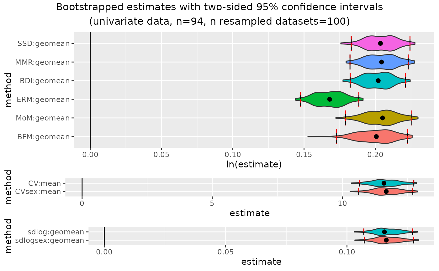
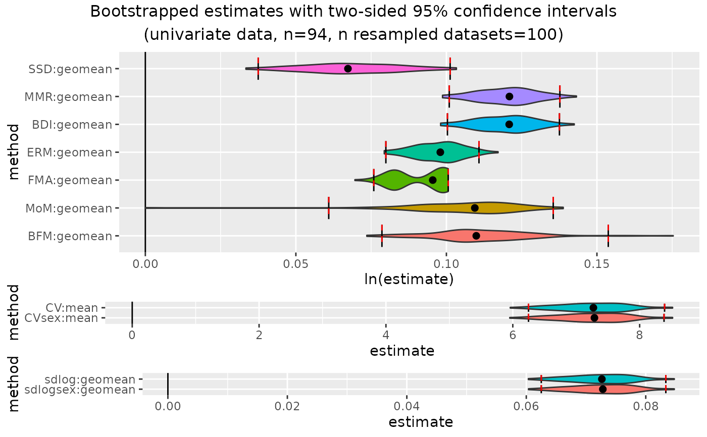
plot(outcomeUgor)
 plot(outcomeUgor, exclude="FMA") # exclude one or more methods from plot
 outcomeUhom
#> dimorphResampledUni Object
#>
#> Comparative data set:
#> number of specimens: 47 female, 47 male
#> number of variables: 1
#> variable name: FHSI
#> SSD estimate methods (univariate):
#> SSD, MMR, BDI, ERM, FMA, MoM, BFM, CV, CVsex, sdlog, sdlogsex
#> Centering algorithms:
#> geometric mean, arithmetic mean
#> Number of unique combinations of univariate method and centering algorithm: 11
#>
#> Resampling data structure:
#> type of resampling: Monte Carlo
#> number of resampled data sets: 100
#> number of individuals in each resampled data set: 94
#> resampling procedure: bootstrap
#> subsamples sampled WITH replacement
#> confidence intervals: two-sided, 95% confidence level
#> other resampling parameters:
#> sex data present
#> ratio variables (if present): natural log of ratio
#> matchvars = FALSE
#> na.rm = TRUE
#>
#> Confidence intervals for estimates:
#> methodUni center lower_lim upper_lim
#> 1 SSD geomean 0.13232427 0.1746887
#> 2 MMR geomean 0.13814458 0.1785132
#> 3 BDI geomean 0.13715205 0.1751541
#> 4 ERM geomean 0.11196729 0.1497382
#> 5 FMA geomean 0.09589985 0.1174456
#> 6 MoM geomean 0.11385003 0.1707368
#> 7 BFM geomean 0.12570338 0.1750055
#> 8 CV mean 8.10843360 10.3599325
#> 9 CVsex mean 8.10843360 10.3187490
#> 10 sdlog geomean 0.08047167 0.1025251
#> 11 sdlogsex geomean 0.08170669 0.1025833
#>
#> Confidence intervals for bias of estimates from sample SSD, CVsex, or sdlogsex:
#> methodUni center lower_lim upper_lim
#> 1 MMR geomean 0.001561279 0.013842138
#> 2 BDI geomean -0.001018798 0.010414694
#> 3 ERM geomean -0.029962929 -0.012656277
#> 4 FMA geomean -0.058768579 -0.016181395
#> 5 MoM geomean -0.020142020 0.006139514
#> 6 BFM geomean -0.010676647 0.012178825
#> 7 CV mean -0.318604951 0.049166961
#> 8 sdlog geomean -0.001691454 0.000000000
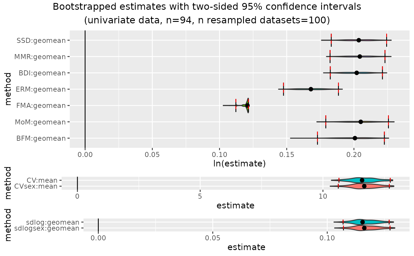
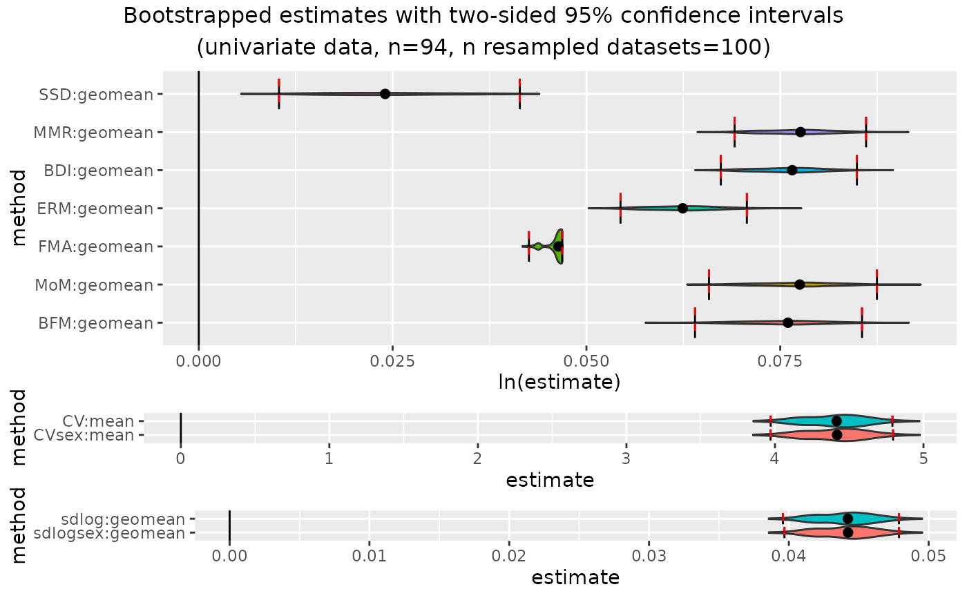
plot(outcomeUhom)
outcomeUhom
#> dimorphResampledUni Object
#>
#> Comparative data set:
#> number of specimens: 47 female, 47 male
#> number of variables: 1
#> variable name: FHSI
#> SSD estimate methods (univariate):
#> SSD, MMR, BDI, ERM, FMA, MoM, BFM, CV, CVsex, sdlog, sdlogsex
#> Centering algorithms:
#> geometric mean, arithmetic mean
#> Number of unique combinations of univariate method and centering algorithm: 11
#>
#> Resampling data structure:
#> type of resampling: Monte Carlo
#> number of resampled data sets: 100
#> number of individuals in each resampled data set: 94
#> resampling procedure: bootstrap
#> subsamples sampled WITH replacement
#> confidence intervals: two-sided, 95% confidence level
#> other resampling parameters:
#> sex data present
#> ratio variables (if present): natural log of ratio
#> matchvars = FALSE
#> na.rm = TRUE
#>
#> Confidence intervals for estimates:
#> methodUni center lower_lim upper_lim
#> 1 SSD geomean 0.13232427 0.1746887
#> 2 MMR geomean 0.13814458 0.1785132
#> 3 BDI geomean 0.13715205 0.1751541
#> 4 ERM geomean 0.11196729 0.1497382
#> 5 FMA geomean 0.09589985 0.1174456
#> 6 MoM geomean 0.11385003 0.1707368
#> 7 BFM geomean 0.12570338 0.1750055
#> 8 CV mean 8.10843360 10.3599325
#> 9 CVsex mean 8.10843360 10.3187490
#> 10 sdlog geomean 0.08047167 0.1025251
#> 11 sdlogsex geomean 0.08170669 0.1025833
#>
#> Confidence intervals for bias of estimates from sample SSD, CVsex, or sdlogsex:
#> methodUni center lower_lim upper_lim
#> 1 MMR geomean 0.001561279 0.013842138
#> 2 BDI geomean -0.001018798 0.010414694
#> 3 ERM geomean -0.029962929 -0.012656277
#> 4 FMA geomean -0.058768579 -0.016181395
#> 5 MoM geomean -0.020142020 0.006139514
#> 6 BFM geomean -0.010676647 0.012178825
#> 7 CV mean -0.318604951 0.049166961
#> 8 sdlog geomean -0.001691454 0.000000000
plot(outcomeUhom)
 outcomeUpan
#> dimorphResampledUni Object
#>
#> Comparative data set:
#> number of specimens: 47 female, 47 male
#> number of variables: 1
#> variable name: FHSI
#> SSD estimate methods (univariate):
#> SSD, MMR, BDI, ERM, FMA, MoM, BFM, CV, CVsex, sdlog, sdlogsex
#> Centering algorithms:
#> geometric mean, arithmetic mean
#> Number of unique combinations of univariate method and centering algorithm: 11
#>
#> Resampling data structure:
#> type of resampling: Monte Carlo
#> number of resampled data sets: 100
#> number of individuals in each resampled data set: 94
#> resampling procedure: bootstrap
#> subsamples sampled WITH replacement
#> confidence intervals: two-sided, 95% confidence level
#> other resampling parameters:
#> sex data present
#> ratio variables (if present): natural log of ratio
#> matchvars = FALSE
#> na.rm = TRUE
#>
#> Confidence intervals for estimates:
#> methodUni center lower_lim upper_lim
#> 1 SSD geomean 0.03749028 0.10123909
#> 2 MMR geomean 0.10095506 0.13769667
#> 3 BDI geomean 0.10033774 0.13754929
#> 4 ERM geomean 0.07989464 0.11081978
#> 5 FMA geomean 0.07588313 0.10061009
#> 6 MoM geomean 0.06091800 0.13548294
#> 7 BFM geomean 0.07858883 0.15376707
#> 8 CV mean 6.24793568 8.39288852
#> 9 CVsex mean 6.24793568 8.38440010
#> 10 sdlog geomean 0.06251004 0.08336113
#> 11 sdlogsex geomean 0.06251004 0.08336113
#>
#> Confidence intervals for bias of estimates from sample SSD, CVsex, or sdlogsex:
#> methodUni center lower_lim upper_lim
#> 1 MMR geomean 0.0290854643 0.07582925
#> 2 BDI geomean 0.0277882372 0.07446179
#> 3 ERM geomean 0.0029249760 0.05242251
#> 4 FMA geomean -0.0112953227 0.05175535
#> 5 MoM geomean -0.0076588667 0.07032486
#> 6 BFM geomean 0.0025312425 0.07986058
#> 7 CV mean -0.0939295045 0.02189832
#> 8 sdlog geomean -0.0004096517 0.00000000
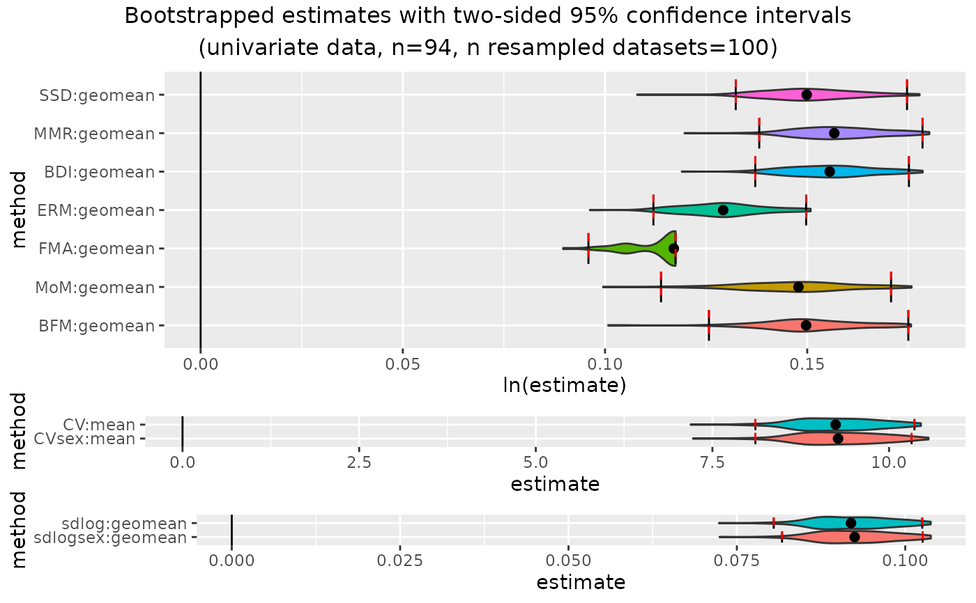
plot(outcomeUpan)
outcomeUpan
#> dimorphResampledUni Object
#>
#> Comparative data set:
#> number of specimens: 47 female, 47 male
#> number of variables: 1
#> variable name: FHSI
#> SSD estimate methods (univariate):
#> SSD, MMR, BDI, ERM, FMA, MoM, BFM, CV, CVsex, sdlog, sdlogsex
#> Centering algorithms:
#> geometric mean, arithmetic mean
#> Number of unique combinations of univariate method and centering algorithm: 11
#>
#> Resampling data structure:
#> type of resampling: Monte Carlo
#> number of resampled data sets: 100
#> number of individuals in each resampled data set: 94
#> resampling procedure: bootstrap
#> subsamples sampled WITH replacement
#> confidence intervals: two-sided, 95% confidence level
#> other resampling parameters:
#> sex data present
#> ratio variables (if present): natural log of ratio
#> matchvars = FALSE
#> na.rm = TRUE
#>
#> Confidence intervals for estimates:
#> methodUni center lower_lim upper_lim
#> 1 SSD geomean 0.03749028 0.10123909
#> 2 MMR geomean 0.10095506 0.13769667
#> 3 BDI geomean 0.10033774 0.13754929
#> 4 ERM geomean 0.07989464 0.11081978
#> 5 FMA geomean 0.07588313 0.10061009
#> 6 MoM geomean 0.06091800 0.13548294
#> 7 BFM geomean 0.07858883 0.15376707
#> 8 CV mean 6.24793568 8.39288852
#> 9 CVsex mean 6.24793568 8.38440010
#> 10 sdlog geomean 0.06251004 0.08336113
#> 11 sdlogsex geomean 0.06251004 0.08336113
#>
#> Confidence intervals for bias of estimates from sample SSD, CVsex, or sdlogsex:
#> methodUni center lower_lim upper_lim
#> 1 MMR geomean 0.0290854643 0.07582925
#> 2 BDI geomean 0.0277882372 0.07446179
#> 3 ERM geomean 0.0029249760 0.05242251
#> 4 FMA geomean -0.0112953227 0.05175535
#> 5 MoM geomean -0.0076588667 0.07032486
#> 6 BFM geomean 0.0025312425 0.07986058
#> 7 CV mean -0.0939295045 0.02189832
#> 8 sdlog geomean -0.0004096517 0.00000000
plot(outcomeUpan)
 outcomeUhyl
#> dimorphResampledUni Object
#>
#> Comparative data set:
#> number of specimens: 47 female, 47 male
#> number of variables: 1
#> variable name: FHSI
#> SSD estimate methods (univariate):
#> SSD, MMR, BDI, ERM, FMA, MoM, BFM, CV, CVsex, sdlog, sdlogsex
#> Centering algorithms:
#> geometric mean, arithmetic mean
#> Number of unique combinations of univariate method and centering algorithm: 11
#>
#> Resampling data structure:
#> type of resampling: Monte Carlo
#> number of resampled data sets: 100
#> number of individuals in each resampled data set: 94
#> resampling procedure: bootstrap
#> subsamples sampled WITH replacement
#> confidence intervals: two-sided, 95% confidence level
#> other resampling parameters:
#> sex data present
#> ratio variables (if present): natural log of ratio
#> matchvars = FALSE
#> na.rm = TRUE
#>
#> Confidence intervals for estimates:
#> methodUni center lower_lim upper_lim
#> 1 SSD geomean 0.01034968 0.04141244
#> 2 MMR geomean 0.06911863 0.08607323
#> 3 BDI geomean 0.06733970 0.08489180
#> 4 ERM geomean 0.05439547 0.07069500
#> 5 FMA geomean 0.04258627 0.04688045
#> 6 MoM geomean 0.06580953 0.08747406
#> 7 BFM geomean 0.06400712 0.08554635
#> 8 CV mean 3.97135539 4.79106663
#> 9 CVsex mean 3.97059559 4.79524126
#> 10 sdlog geomean 0.03957947 0.04787749
#> 11 sdlogsex geomean 0.03968688 0.04788334
#>
#> Confidence intervals for bias of estimates from sample SSD, CVsex, or sdlogsex:
#> methodUni center lower_lim upper_lim
#> 1 MMR geomean 3.756253e-02 0.068574973
#> 2 BDI geomean 3.673327e-02 0.067393545
#> 3 ERM geomean 2.351016e-02 0.053284699
#> 4 FMA geomean 5.468008e-03 0.035253518
#> 5 MoM geomean 3.776905e-02 0.069975801
#> 6 BFM geomean 3.585783e-02 0.068191870
#> 7 CV mean -1.506556e-02 0.004373101
#> 8 sdlog geomean -9.627827e-05 0.000000000
plot(outcomeUhyl)
outcomeUhyl
#> dimorphResampledUni Object
#>
#> Comparative data set:
#> number of specimens: 47 female, 47 male
#> number of variables: 1
#> variable name: FHSI
#> SSD estimate methods (univariate):
#> SSD, MMR, BDI, ERM, FMA, MoM, BFM, CV, CVsex, sdlog, sdlogsex
#> Centering algorithms:
#> geometric mean, arithmetic mean
#> Number of unique combinations of univariate method and centering algorithm: 11
#>
#> Resampling data structure:
#> type of resampling: Monte Carlo
#> number of resampled data sets: 100
#> number of individuals in each resampled data set: 94
#> resampling procedure: bootstrap
#> subsamples sampled WITH replacement
#> confidence intervals: two-sided, 95% confidence level
#> other resampling parameters:
#> sex data present
#> ratio variables (if present): natural log of ratio
#> matchvars = FALSE
#> na.rm = TRUE
#>
#> Confidence intervals for estimates:
#> methodUni center lower_lim upper_lim
#> 1 SSD geomean 0.01034968 0.04141244
#> 2 MMR geomean 0.06911863 0.08607323
#> 3 BDI geomean 0.06733970 0.08489180
#> 4 ERM geomean 0.05439547 0.07069500
#> 5 FMA geomean 0.04258627 0.04688045
#> 6 MoM geomean 0.06580953 0.08747406
#> 7 BFM geomean 0.06400712 0.08554635
#> 8 CV mean 3.97135539 4.79106663
#> 9 CVsex mean 3.97059559 4.79524126
#> 10 sdlog geomean 0.03957947 0.04787749
#> 11 sdlogsex geomean 0.03968688 0.04788334
#>
#> Confidence intervals for bias of estimates from sample SSD, CVsex, or sdlogsex:
#> methodUni center lower_lim upper_lim
#> 1 MMR geomean 3.756253e-02 0.068574973
#> 2 BDI geomean 3.673327e-02 0.067393545
#> 3 ERM geomean 2.351016e-02 0.053284699
#> 4 FMA geomean 5.468008e-03 0.035253518
#> 5 MoM geomean 3.776905e-02 0.069975801
#> 6 BFM geomean 3.585783e-02 0.068191870
#> 7 CV mean -1.506556e-02 0.004373101
#> 8 sdlog geomean -9.627827e-05 0.000000000
plot(outcomeUhyl)
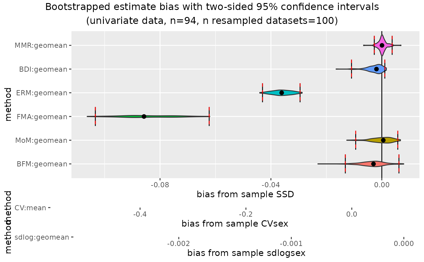
 confint(outcomeUgor, type="bias")
#> methodUni center lower_lim0.95 upper_lim0.95
#> 1 MMR geomean -0.002714140 0.0037295781
#> 2 BDI geomean -0.010926772 0.0010901125
#> 3 ERM geomean -0.043033344 -0.0294849908
#> 4 FMA geomean -0.103335017 -0.0622690871
#> 5 MoM geomean -0.009424754 0.0057562290
#> 6 BFM geomean -0.013164757 0.0061751930
#> 7 CV mean -0.395708367 0.0913325678
#> 8 sdlog geomean -0.002414336 -0.0000184736
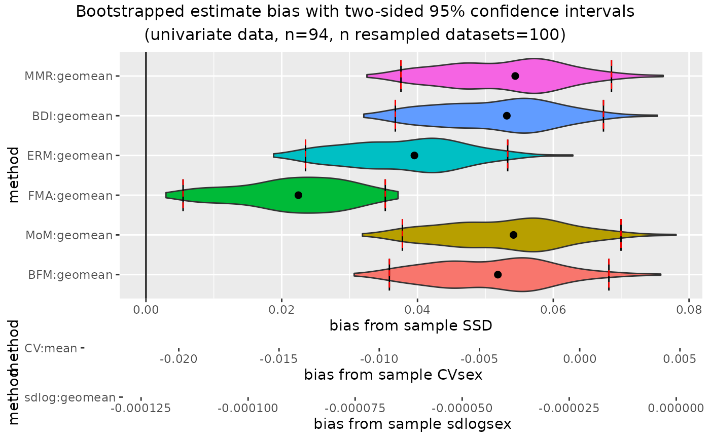
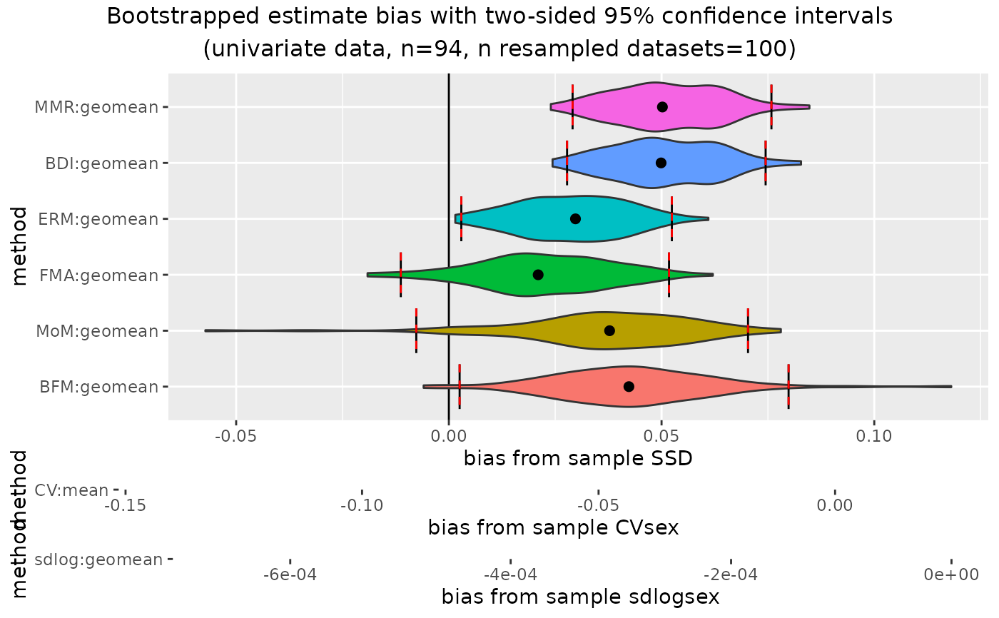
plot(outcomeUgor, type="bias")
confint(outcomeUgor, type="bias")
#> methodUni center lower_lim0.95 upper_lim0.95
#> 1 MMR geomean -0.002714140 0.0037295781
#> 2 BDI geomean -0.010926772 0.0010901125
#> 3 ERM geomean -0.043033344 -0.0294849908
#> 4 FMA geomean -0.103335017 -0.0622690871
#> 5 MoM geomean -0.009424754 0.0057562290
#> 6 BFM geomean -0.013164757 0.0061751930
#> 7 CV mean -0.395708367 0.0913325678
#> 8 sdlog geomean -0.002414336 -0.0000184736
plot(outcomeUgor, type="bias")
 plot(outcomeUhom, type="bias")
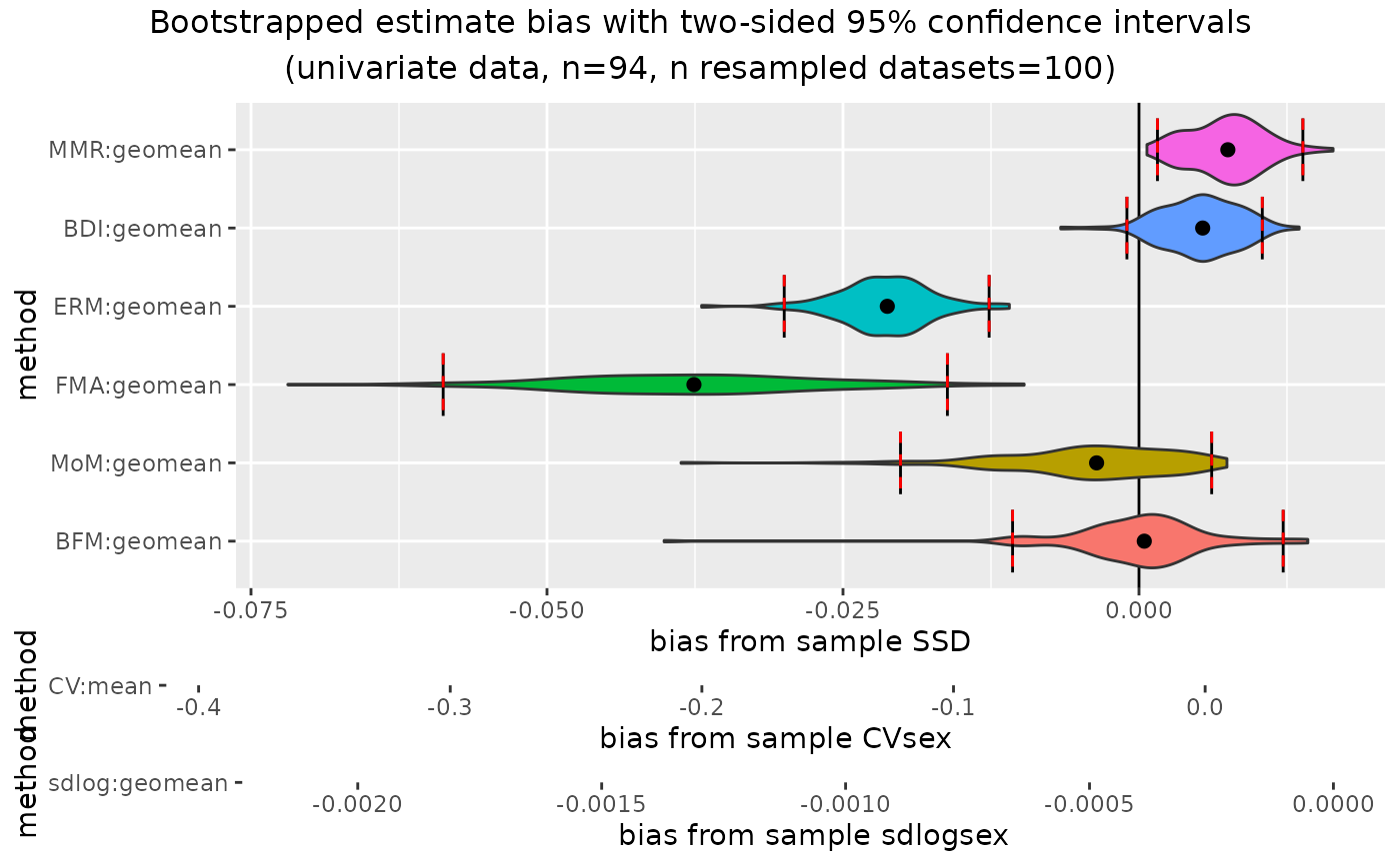 plot(outcomeUpan, type="bias")
 plot(outcomeUhyl, type="bias")