Significance Tests for Sexual Size Dimorphism Estimates
SSDtest.RdFunction to calculate p-values for pairwise comparisons of dimorphism estimates for two or more univariate
or multivariate samples. The first step in this process identifies the minimum sample size (and missing data
structure) present in the samples of fossil; for multivariate datasets with missing data, datasets are
restricted to individuals with measurements in variables present in all samples. All datasets are then resampled to
the sample size (and missing data structure) of the minimum sample. This function generates both
two-sided and one-sided p-values for each pair of samples.
Usage
SSDtest(
  fossil = NULL,
  comp = NULL,
  fossilsex = NULL,
  compsex = NULL,
  methsUni = c("MMR", "BDI"),
  methsMulti = "GMM",
  replace = F,
  rebootstrap = F,
  fullsamplesboot = F,
  nResamp = 1000,
  exactcomp = T,
  exactfossil = T,
  limit = 50000,
  center = "geomean",
  sex.female = 1,
  na.rm = T,
  ncorrection = F,
  matchvars = F,
  datastruc = NULL,
  templatevar = NULL
)
Arguments
- fossil
A list of matrices or data frames of measurements from fossil sample(s) (or other test samples) to be compared in a series of pairwise resampling tests, with rows corresponding to individual specimens and columns corresponding to size variables. Sex data should not be included. Some data can be missing. When a single fossil sample is present, by default null distributions of resampled values from comparative data sets will be compared to a single point estimate generated for the fossil sample (one point estimate per estimation method).
fossilmay beNULL, in which case all samples should be provided incomp, and all samples will be resampled.- comp
A list of matrices or data frames of measurements from comparative sample(s) to be compared in a series of pairwise resampling tests, with rows corresponding to individual specimens and columns corresponding to size variables. Sex data should not be included. All data sets must be complete for all measurements.
- fossilsex
A list of vectors indicating sex for the individuals in each of the samples in
fossil. Defaults toNULL.- compsex
A list of vectors indicating sex for the individuals in each of the samples in
comp. Defaults toNULL.- methsUni
A character vector specifying the univariate method(s) used to calculate or estimate dimorphism. See
dimorphfor options. Defaults toc("MMR", "BDI").- methsMulti
A character vector specifying the multivariate method(s) used to calculate or estimate dimorphism. Note that regardless of the value of this argument, multivariate estimation procedures will only be carried out if
fossilandcompare multivariate datasets. Seedimorphfor options. Defaults to"GMM".- replace
Logical scalar specifying whether to sample from comparative datasets with replacement or not. Defaults to
FALSE.- rebootstrap
Logical scalar specifying whether to add an additional step after initial resampling in which resampled addresses for both comparative and fossil datasets are bootstrapped (i.e., sampled with replacement to an equal sample sizes as the initial set of resampled addresses). This procedure implements the highly conservative "resampled extinct distribution method" of Gordon et al. (2008). Defaults to
FALSE. Warning: settingrebootstraptoTRUEwill drastically reduce power!- fullsamplesboot
Logical scalar. If all samples are complete (no missing data) and
fullsamplesbootis set toTRUE, rather than downsampling to the minimum sample infossil, all samples infossilare andcompare bootstrapped (i.e., sampled with replacement at their full sample size). Defaults toFALSE. Note that for univariate analyses,NAs are removed by default so all datasets (including fossils) are considered complete. Therefore settingfullsamplesboottoTRUEfor univariate analyses with fossils will bootstrap the fossil dataset rather than generating a single point estimate from the fossil dataset.- nResamp
Integer specifying the number of resampling iterations if Monte Carlo sampling is used. Defaults to
1,000.- exactcomp
Logical scalar specifying for samples in
compwhether to sample all possible unique combinations of resampled datasets for the minimum data structure present infossil. If set toFALSE, or if set toTRUEand the number of unique combinations exceedslimit, then Monte Carlo sampling is used instead. Defaults toTRUE.- exactfossil
Logical scalar specifying for samples in
fossilwhether to sample all possible unique combinations of resampled datasets for the minimum data structure present infossil. If set toFALSE, or if set toTRUEand the number of unique combinations exceedslimit, then Monte Carlo sampling is used instead. Defaults toTRUE.- limit
Integer setting the upper limit on the number of unique combinations allowable for exact resampling. If exact resampling would produce more resampled datasets than this number, Monte Carlo resampling is used instead. Defaults to
50,000.- center
A character string specifying the method used to calculate a mean, either
"geomean"(default) which uses the geometric mean, or"mean"which uses the arithmetic mean. More broadly,"geomean"indicates analyses are conducted in logarithmic data space and"mean"indicates analyses are conducted in raw data space. Some methods can only be applied in one domain or the other:"CV"and"CVsex"are always calculated in raw data space andcenterwill be set to"mean"for these methods regardless of the value set by the user;"MoM","sdlog", and"sdlogsex"are always calculated in logarithmic data space andcenterwill be set to"geomean"for these methods regardless of the value set by the user.- sex.female
An integer scalar (1 or 2) specifying which level of
sexcorresponds to female. Ignored ifsexisNULL. Defaults to 1.- na.rm
A logical scalar indicating whether
NAvalues should be stripped before the computation proceeds in univariate analyses. Not relevant for multivariate analyses. Defaults toTRUE.- ncorrection
A logical scalar indicating whether to apply Sokal and Braumann's (1980) size correction factor to CV estimates. Defaults to
FALSE.- matchvars
Logical scalar specifying whether to compare the shared set of variable names in
compandfossilto the variable names instrucand pare them all down to the set of shared variables. IfFALSEand variable names differ then an error will be returned. Defaults toFALSE.- datastruc
If multivariate data are used, this is a character string specifiying whether to incorporate the missing data structure into dimorphism estimates (
"missing"), whether to downsample to the missing data sample size but keep all metric data for the comparative sample ("complete"), or to perform both types of resampling separately ("both"). Ignored if only univariate data are provided or if all datasets are complete. Defaults toNULL, which reverts to"missing"if some datasets are incomplete.- templatevar
A character object or integer value specifying the name or column number of the variable in
fossilandcompto be estimated using the template method. Ignored if template method is not used. Defaults toNULL.
Value
A list of class SSDtest. Printing this object provides information about the datasets and
test performed, median values for resampled distributions for each sample for each method used, confidence
intervals for all estimators calculated, and calculated p-values. Plotting this object produces
histograms for resampled distributions for one or more estimation methods, or histograms for differences
between samples (see plot.SSDtest).
References
Gordon AD, Green DJ, Richmond BG. (2008) Strong postcranial size dimorphism in Australopithecus afarensis: Results from two new resampling methods for multivariate data sets with missing data. American Journal of Physical Anthropology. 135:311-328. (https://doi.org/10.1002/ajpa.20745)
Examples
# SSDtests using simulated fossils generated from real gorilla and human samples with some
# data removed
data(fauxil)
fauxil
#> Species Museum Collection.ID FHSI TPML TPMAP TPLAP HHMaj
#> PCM Gg-M877 Fauxil sp. 1 PCM Gg-M877 NA NA 40.71 NA NA
#> PCM Gg-Z6-33 Fauxil sp. 1 PCM Gg-Z6-33 NA 69.42 NA NA 46.18
#> CMNH HTB 1997 Fauxil sp. 1 CMNH HTB 1997 NA NA NA NA 50.86
#> CMNH HTB 1710 Fauxil sp. 1 CMNH HTB 1710 39.85 66.34 41.42 NA NA
#> CMNH HTB 1846 Fauxil sp. 1 CMNH HTB 1846 NA NA NA 32.39 49.47
#> CMNH HTB 1851 Fauxil sp. 1 CMNH HTB 1851 NA NA NA 37.26 NA
#> ZSM 1954/0201 Fauxil sp. 1 ZSM 1954/0201 NA NA NA NA NA
#> MNHN 1982-56 Fauxil sp. 1 MNHN 1982-56 NA NA NA NA NA
#> CMNH HTB 1729 Fauxil sp. 1 CMNH HTB 1729 47.93 NA NA NA NA
#> PCM Gg-C1-105 Fauxil sp. 1 PCM Gg-C1-105 NA NA NA NA NA
#> CMNH HTB 1994 Fauxil sp. 1 CMNH HTB 1994 49.68 NA NA 46.94 60.95
#> CMNH HTB 1732 Fauxil sp. 1 CMNH HTB 1732 NA NA NA 40.46 NA
#> CMNH HTB 1954 Fauxil sp. 1 CMNH HTB 1954 NA NA NA NA NA
#> CMNH HTB 1797 Fauxil sp. 1 CMNH HTB 1797 NA NA NA NA 66.85
#> MNHN 1931-657 Fauxil sp. 1 MNHN 1931-657 53.17 86.29 NA NA NA
#> CMNH HTB 3400 Fauxil sp. 1 CMNH HTB 3400 NA 93.74 NA NA NA
#> CMNH HTH 1709 Fauxil sp. 2 CMNH HTH 1709 39.73 NA NA NA NA
#> CMNH HTH 1779 Fauxil sp. 2 CMNH HTH 1779 NA NA NA NA 40.01
#> CMNH HTH 0221 Fauxil sp. 2 CMNH HTH 0221 NA NA NA 36.78 NA
#> CMNH HTH 1270 Fauxil sp. 2 CMNH HTH 1270 41.80 NA 46.30 NA 40.16
#> CMNH HTH 2056 Fauxil sp. 2 CMNH HTH 2056 43.86 NA 45.85 NA NA
#> CMNH HTH 2761 Fauxil sp. 2 CMNH HTH 2761 NA 72.32 NA NA 41.46
#> CMNH HTH 0727 Fauxil sp. 2 CMNH HTH 0727 NA NA 50.17 NA NA
#> CMNH HTH 1755 Fauxil sp. 2 CMNH HTH 1755 44.91 NA NA NA NA
#> CMNH HTH 2428 Fauxil sp. 2 CMNH HTH 2428 45.32 NA NA NA 45.66
#> CMNH HTH 1685 Fauxil sp. 2 CMNH HTH 1685 NA NA 47.52 NA 46.81
#> CMNH HTH 0383 Fauxil sp. 2 CMNH HTH 0383 NA NA NA NA NA
#> CMNH HTH 0280 Fauxil sp. 2 CMNH HTH 0280 47.46 NA 44.99 NA NA
#> CMNH HTH 0922 Fauxil sp. 2 CMNH HTH 0922 47.48 NA NA NA NA
#> CMNH HTH 0878 Fauxil sp. 2 CMNH HTH 0878 NA NA NA 44.17 NA
#> CMNH HTH 1398 Fauxil sp. 2 CMNH HTH 1398 NA NA NA 42.80 NA
#> CMNH HTH 2584 Fauxil sp. 2 CMNH HTH 2584 NA NA NA NA NA
#> CMNH HTH 1389 Fauxil sp. 2 CMNH HTH 1389 49.30 NA NA NA NA
#> CMNH HTH 0720 Fauxil sp. 2 CMNH HTH 0720 NA 76.92 NA NA NA
#> CMNH HTH 0712 Fauxil sp. 2 CMNH HTH 0712 NA NA NA 44.53 NA
#> HHMin RHMaj RHMin RDAP RDML
#> PCM Gg-M877 NA NA 25.67 NA NA
#> PCM Gg-Z6-33 NA NA NA NA 28.87
#> CMNH HTB 1997 42.31 NA NA NA NA
#> CMNH HTB 1710 43.04 NA 24.72 19.63 NA
#> CMNH HTB 1846 44.10 NA NA NA NA
#> CMNH HTB 1851 NA NA NA 20.79 NA
#> ZSM 1954/0201 NA 26.83 26.00 NA NA
#> MNHN 1982-56 NA NA 30.50 NA NA
#> CMNH HTB 1729 NA NA NA 26.68 NA
#> PCM Gg-C1-105 59.26 NA NA NA 36.06
#> CMNH HTB 1994 NA 34.65 NA NA NA
#> CMNH HTB 1732 56.03 NA NA NA NA
#> CMNH HTB 1954 57.52 NA NA NA NA
#> CMNH HTB 1797 NA NA NA NA NA
#> MNHN 1931-657 NA NA NA NA NA
#> CMNH HTB 3400 NA NA NA NA NA
#> CMNH HTH 1709 NA NA NA 13.82 NA
#> CMNH HTH 1779 NA NA NA NA 26.13
#> CMNH HTH 0221 NA NA NA NA NA
#> CMNH HTH 1270 NA NA NA NA NA
#> CMNH HTH 2056 NA NA NA NA NA
#> CMNH HTH 2761 NA NA NA 13.79 NA
#> CMNH HTH 0727 NA NA NA NA NA
#> CMNH HTH 1755 NA NA NA NA 28.89
#> CMNH HTH 2428 NA 23.39 NA 14.53 NA
#> CMNH HTH 1685 NA 26.30 NA NA NA
#> CMNH HTH 0383 NA 21.04 NA NA 27.48
#> CMNH HTH 0280 NA NA NA NA NA
#> CMNH HTH 0922 NA NA NA NA NA
#> CMNH HTH 0878 NA NA NA NA NA
#> CMNH HTH 1398 44.71 NA NA NA NA
#> CMNH HTH 2584 NA NA NA NA 30.52
#> CMNH HTH 1389 NA NA NA NA NA
#> CMNH HTH 0720 NA NA NA NA NA
#> CMNH HTH 0712 47.62 NA NA NA 32.15
## Univariate examples
# First, some code that would generate errors
# SSDtest()
# SSDtest(fossil=list("Fauxil sp. 1"=fauxil[fauxil$Species=="Fauxil sp. 1", "FHSI"]))
# SSDtest(comp=list("G. gorilla"=apelimbart[apelimbart$Species=="Gorilla gorilla", "FHSI"]))
# Standard significance test with one fossil sample, sampling without replacement
test_faux_uni <- SSDtest(
fossil=list("Fauxil sp. 1"=fauxil[fauxil$Species=="Fauxil sp. 1", "FHSI"]),
comp=list("G. gorilla"=apelimbart[apelimbart$Species=="Gorilla gorilla", "FHSI"],
"H. sapiens"=apelimbart[apelimbart$Species=="Homo sapiens", "FHSI"],
"P. troglodytes"=apelimbart[apelimbart$Species=="Pan troglodytes", "FHSI"],
"H. lar"=apelimbart[apelimbart$Species=="Hylobates lar", "FHSI"]),
fossilsex=NULL,
compsex=list("G. gorilla"=apelimbart[apelimbart$Species=="Gorilla gorilla", "Sex"],
"H. sapiens"=apelimbart[apelimbart$Species=="Homo sapiens", "Sex"],
"P. troglodytes"=apelimbart[apelimbart$Species=="Pan troglodytes", "Sex"],
"H. lar"=apelimbart[apelimbart$Species=="Hylobates lar", "Sex"]),
methsUni=c("SSD", "MMR", "BDI"),
limit=1000,
nResamp=100)
#> Warning: The number of possible combinations (3049501) exceeds the user-specified limit. Monte Carlo sampling will be used.
#> Warning: The number of possible combinations (3049501) exceeds the user-specified limit. Monte Carlo sampling will be used.
#> Warning: The number of possible combinations (3049501) exceeds the user-specified limit. Monte Carlo sampling will be used.
#> Warning: The number of possible combinations (3049501) exceeds the user-specified limit. Monte Carlo sampling will be used.
#> Warning: The following comparisons contain NAs that were
#> dropped in the calculation of p-values:
#> SSD:geomean: G. gorilla - H. sapiens
#> SSD:geomean: G. gorilla - P. troglodytes
#> SSD:geomean: G. gorilla - H. lar
#> SSD:geomean: H. sapiens - P. troglodytes
#> SSD:geomean: H. sapiens - H. lar
#> SSD:geomean: P. troglodytes - H. lar
#> SSD:geomean: H. sapiens - G. gorilla
#> SSD:geomean: P. troglodytes - G. gorilla
#> SSD:geomean: H. lar - G. gorilla
#> SSD:geomean: P. troglodytes - H. sapiens
#> SSD:geomean: H. lar - H. sapiens
#> SSD:geomean: H. lar - P. troglodytes
test_faux_uni
#> SSDtest Object
#>
#> Comparative data set:
#> sample n female n male n unspecified
#> Fauxil sp. 1 0 0 4
#> G. gorilla 47 47 0
#> H. sapiens 47 47 0
#> P. troglodytes 47 47 0
#> H. lar 47 47 0
#> number of variables: 1
#> variable names: VAR
#> SSD estimate methods (univariate):
#> SSD, MMR, BDI
#> Centering algorithms:
#> geometric mean
#> Number of unique combinations of univariate method and centering algorithm: 3
#>
#> Resampling data structure:
#> sample n resampled data sets resampling type sampling
#> Fauxil sp. 1 1 exact without replacement
#> G. gorilla 100 Monte Carlo without replacement
#> H. sapiens 100 Monte Carlo without replacement
#> P. troglodytes 100 Monte Carlo without replacement
#> H. lar 100 Monte Carlo without replacement
#> number of individuals in each resampled data set: 4
#> other resampling parameters:
#> ratio variables (if present): natural log of ratio
#> matchvars = FALSE
#> na.rm = TRUE
#>
#> Median resampled estimates for each combination of methods:
#> methodUni center Fauxil sp. 1 G. gorilla H. sapiens P. troglodytes H. lar
#> 1 SSD geomean NA 0.1986 0.1538 0.0756 0.0248
#> 2 MMR geomean 0.2312 0.1875 0.1509 0.1275 0.0757
#> 3 BDI geomean 0.1793 0.1685 0.1291 0.1031 0.0656
#>
#> p-values (one-sided; null: first sample less or equally dimorphic as second sample):
#> SSD:geomean MMR:geomean BDI:geomean
#> Fauxil sp. 1 - G. gorilla NA 0.2600 0.4300
#> Fauxil sp. 1 - H. sapiens NA 0.1100 0.1700
#> Fauxil sp. 1 - P. troglodytes NA 0.0100 0.0300
#> Fauxil sp. 1 - H. lar NA 0.0000 0.0000
#> G. gorilla - H. sapiens 0.3140 0.3584 0.3140
#> G. gorilla - P. troglodytes 0.0643 0.2251 0.1885
#> G. gorilla - H. lar 0.0027 0.0555 0.0379
#> H. sapiens - P. troglodytes 0.1902 0.3632 0.3573
#> H. sapiens - H. lar 0.0670 0.1322 0.1279
#> P. troglodytes - H. lar 0.2674 0.2209 0.2031
#> G. gorilla - Fauxil sp. 1 NA 0.7400 0.5700
#> H. sapiens - Fauxil sp. 1 NA 0.8900 0.8300
#> P. troglodytes - Fauxil sp. 1 NA 0.9900 0.9700
#> H. lar - Fauxil sp. 1 NA 1.0000 1.0000
#> H. sapiens - G. gorilla 0.6860 0.6416 0.6860
#> P. troglodytes - G. gorilla 0.9357 0.7749 0.8115
#> H. lar - G. gorilla 0.9973 0.9445 0.9621
#> P. troglodytes - H. sapiens 0.8098 0.6368 0.6427
#> H. lar - H. sapiens 0.9330 0.8678 0.8721
#> H. lar - P. troglodytes 0.7326 0.7791 0.7969
#>
#> p-values (two-sided):
#> SSD:geomean MMR:geomean BDI:geomean
#> Fauxil sp. 1 - G. gorilla NA 0.4800 0.8300
#> Fauxil sp. 1 - H. sapiens NA 0.2400 0.3700
#> Fauxil sp. 1 - P. troglodytes NA 0.0100 0.0700
#> Fauxil sp. 1 - H. lar NA 0.0000 0.0000
#> G. gorilla - H. sapiens 0.6149 0.7268 0.6430
#> G. gorilla - P. troglodytes 0.1399 0.4522 0.3729
#> G. gorilla - H. lar 0.0110 0.1029 0.0672
#> H. sapiens - P. troglodytes 0.3791 0.7099 0.7018
#> H. sapiens - H. lar 0.1259 0.2576 0.2477
#> P. troglodytes - H. lar 0.5522 0.4374 0.3972
#>
#> Warning: The following comparisons contain NAs that were
#> dropped in the calculation of p-values:
#> SSD:geomean: G. gorilla - H. sapiens
#> SSD:geomean: G. gorilla - P. troglodytes
#> SSD:geomean: G. gorilla - H. lar
#> SSD:geomean: H. sapiens - P. troglodytes
#> SSD:geomean: H. sapiens - H. lar
#> SSD:geomean: P. troglodytes - H. lar
#> SSD:geomean: H. sapiens - G. gorilla
#> SSD:geomean: P. troglodytes - G. gorilla
#> SSD:geomean: H. lar - G. gorilla
#> SSD:geomean: P. troglodytes - H. sapiens
#> SSD:geomean: H. lar - H. sapiens
#> SSD:geomean: H. lar - P. troglodytes
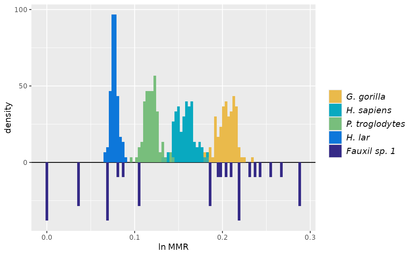
plot(test_faux_uni) # plots first method by default (SSD)
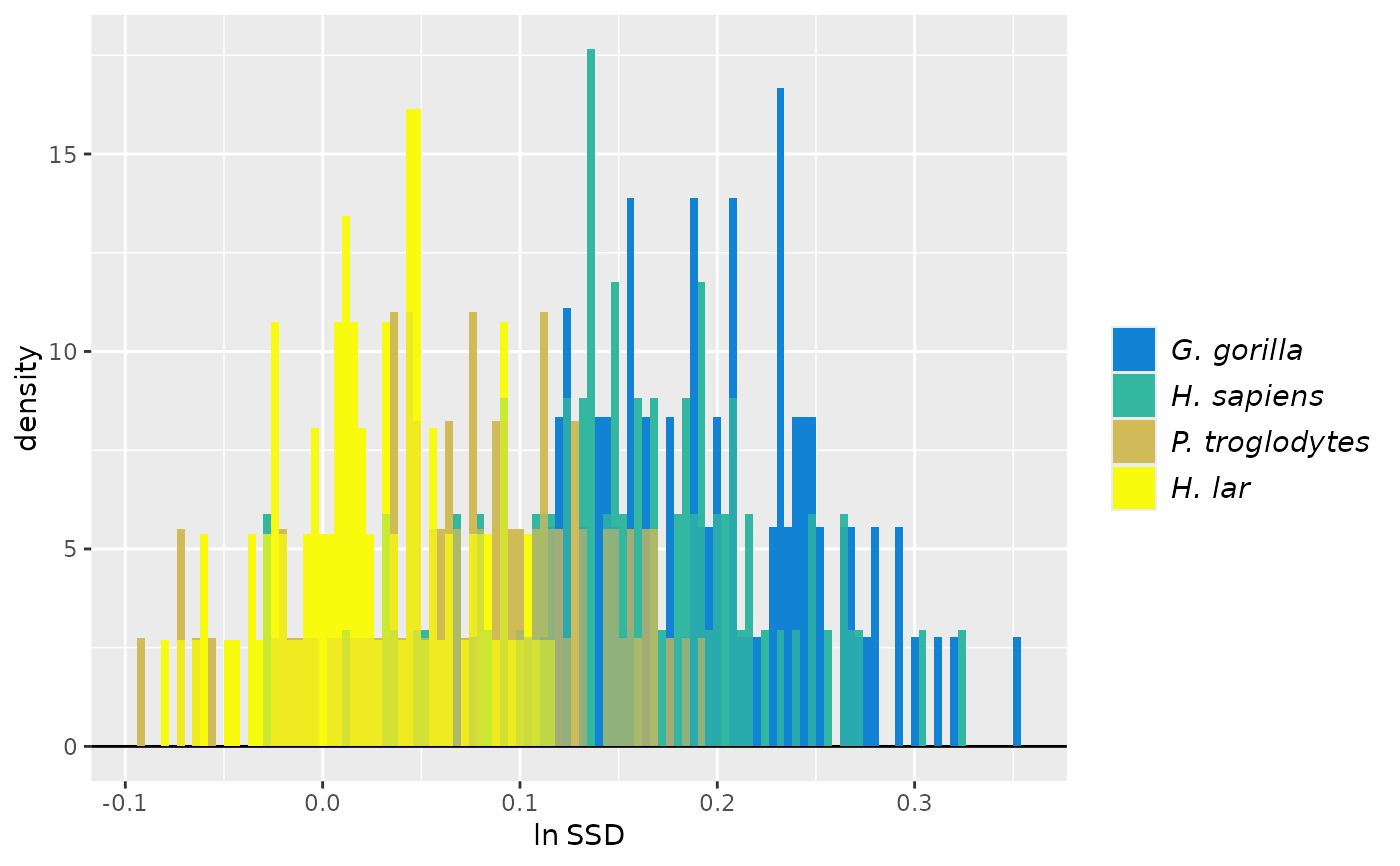 plot(test_faux_uni, est=2) # plots second method (MMR)
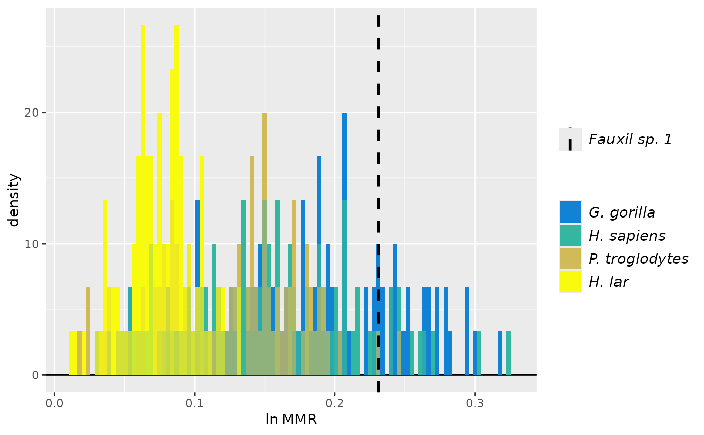 speciescolors <- c("Fauxil sp. 1"="#352A87", "Fauxil sp. 2"="#F9FB0E", "G. gorilla"="#EABA4B",
"H. sapiens"="#09A9C0", "P. troglodytes"="#78BE7C", "H. lar"="#0D77DA")
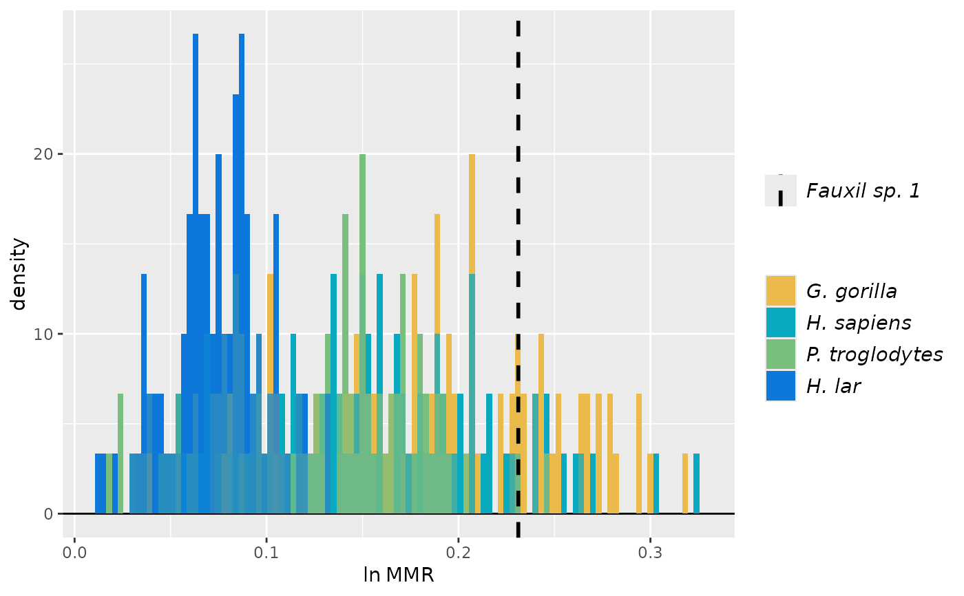
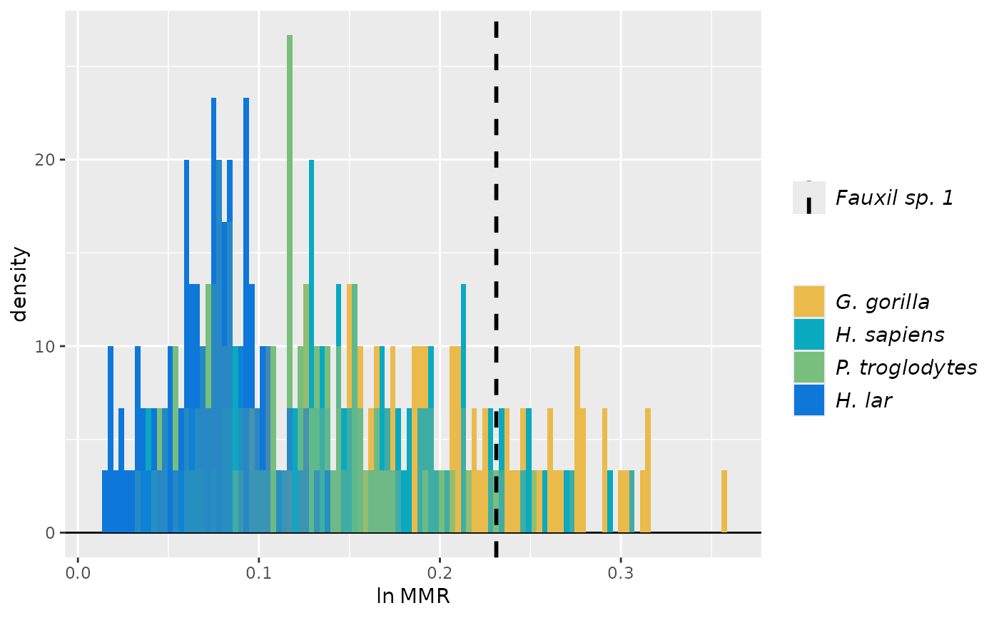
plot(test_faux_uni, est=2, groupcols=speciescolors) # change the colors
speciescolors <- c("Fauxil sp. 1"="#352A87", "Fauxil sp. 2"="#F9FB0E", "G. gorilla"="#EABA4B",
"H. sapiens"="#09A9C0", "P. troglodytes"="#78BE7C", "H. lar"="#0D77DA")
plot(test_faux_uni, est=2, groupcols=speciescolors) # change the colors
 plot(test_faux_uni, type="diff", est=2) # plots differences between samples
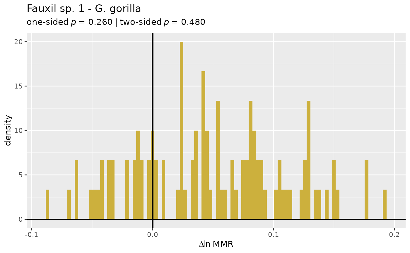
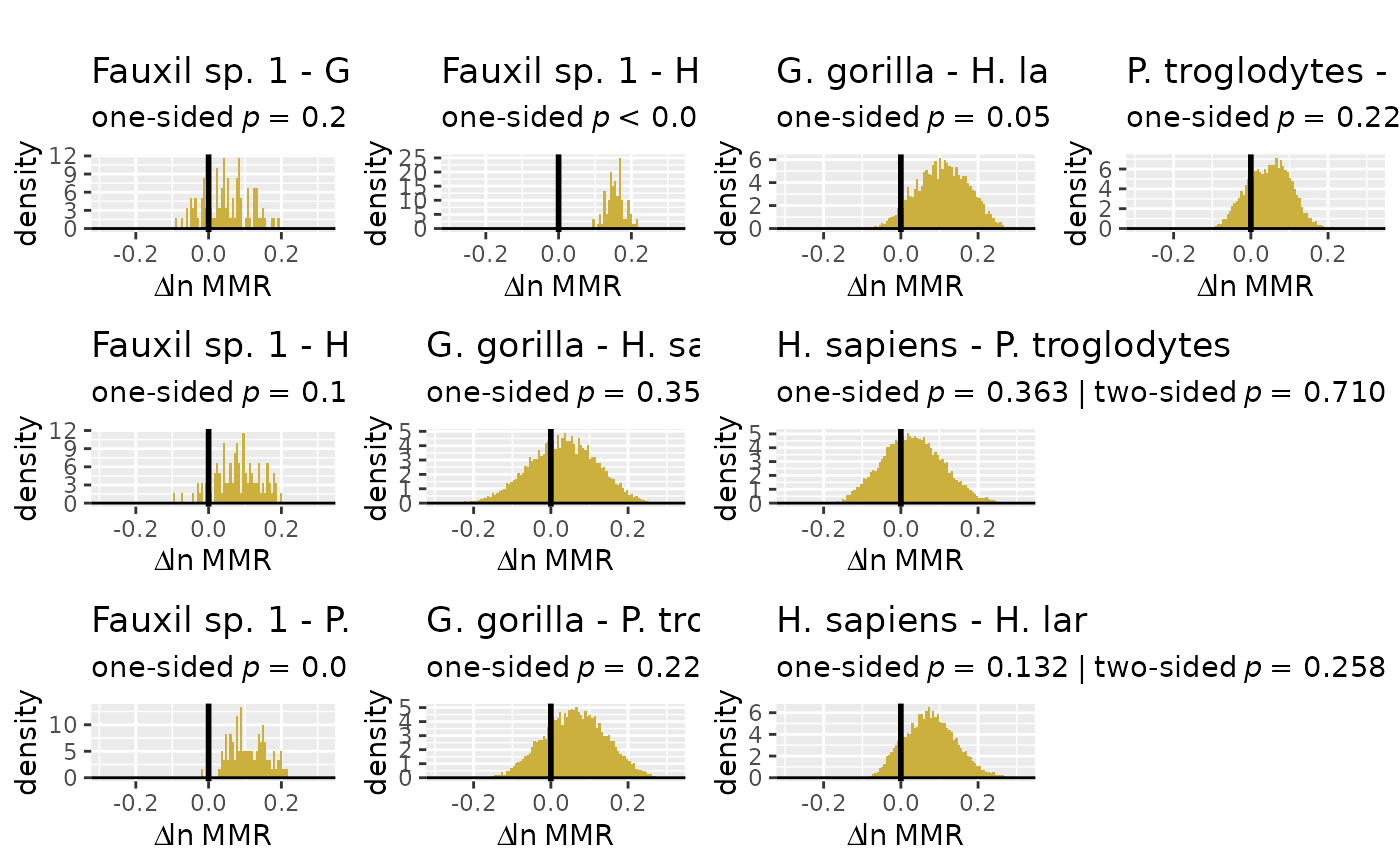 plot(test_faux_uni, type="diff", est=2, diffs=c(1,2)) # plots diffs between first pair of samples
 # Same as above, but variable name information is preserved
test_faux_uni2 <- SSDtest(
fossil=list("Fauxil sp. 1"=fauxil[fauxil$Species=="Fauxil sp. 1", "FHSI", drop=FALSE]),
comp=list("G. gorilla"=apelimbart[apelimbart$Species=="Gorilla gorilla", "FHSI", drop=FALSE],
"H. sapiens"=apelimbart[apelimbart$Species=="Homo sapiens", "FHSI", drop=FALSE],
"P. troglodytes"=apelimbart[apelimbart$Species=="Pan troglodytes","FHSI",drop=FALSE],
"H. lar"=apelimbart[apelimbart$Species=="Hylobates lar", "FHSI", drop=FALSE]),
fossilsex=NULL,
compsex=list("G. gorilla"=apelimbart[apelimbart$Species=="Gorilla gorilla", "Sex"],
"H. sapiens"=apelimbart[apelimbart$Species=="Homo sapiens", "Sex"],
"P. troglodytes"=apelimbart[apelimbart$Species=="Pan troglodytes", "Sex"],
"H. lar"=apelimbart[apelimbart$Species=="Hylobates lar", "Sex"]),
methsUni=c("SSD", "MMR", "BDI"),
limit=1000,
nResamp=100)
#> Warning: The number of possible combinations (3049501) exceeds the user-specified limit. Monte Carlo sampling will be used.
#> Warning: The number of possible combinations (3049501) exceeds the user-specified limit. Monte Carlo sampling will be used.
#> Warning: The number of possible combinations (3049501) exceeds the user-specified limit. Monte Carlo sampling will be used.
#> Warning: The number of possible combinations (3049501) exceeds the user-specified limit. Monte Carlo sampling will be used.
#> Warning: The following comparisons contain NAs that were
#> dropped in the calculation of p-values:
#> SSD:geomean: G. gorilla - H. sapiens
#> SSD:geomean: G. gorilla - P. troglodytes
#> SSD:geomean: G. gorilla - H. lar
#> SSD:geomean: H. sapiens - P. troglodytes
#> SSD:geomean: H. sapiens - H. lar
#> SSD:geomean: P. troglodytes - H. lar
#> SSD:geomean: H. sapiens - G. gorilla
#> SSD:geomean: P. troglodytes - G. gorilla
#> SSD:geomean: H. lar - G. gorilla
#> SSD:geomean: P. troglodytes - H. sapiens
#> SSD:geomean: H. lar - H. sapiens
#> SSD:geomean: H. lar - P. troglodytes
test_faux_uni2
#> SSDtest Object
#>
#> Comparative data set:
#> sample n female n male n unspecified
#> Fauxil sp. 1 0 0 4
#> G. gorilla 47 47 0
#> H. sapiens 47 47 0
#> P. troglodytes 47 47 0
#> H. lar 47 47 0
#> number of variables: 1
#> variable names: FHSI
#> SSD estimate methods (univariate):
#> SSD, MMR, BDI
#> Centering algorithms:
#> geometric mean
#> Number of unique combinations of univariate method and centering algorithm: 3
#>
#> Resampling data structure:
#> sample n resampled data sets resampling type sampling
#> Fauxil sp. 1 1 exact without replacement
#> G. gorilla 100 Monte Carlo without replacement
#> H. sapiens 100 Monte Carlo without replacement
#> P. troglodytes 100 Monte Carlo without replacement
#> H. lar 100 Monte Carlo without replacement
#> number of individuals in each resampled data set: 4
#> other resampling parameters:
#> ratio variables (if present): natural log of ratio
#> matchvars = FALSE
#> na.rm = TRUE
#>
#> Median resampled estimates for each combination of methods:
#> methodUni center Fauxil sp. 1 G. gorilla H. sapiens P. troglodytes H. lar
#> 1 SSD geomean NA 0.1954 0.1511 0.0651 0.0408
#> 2 MMR geomean 0.2312 0.1904 0.1451 0.1083 0.0757
#> 3 BDI geomean 0.1793 0.1590 0.1291 0.0912 0.0650
#>
#> p-values (one-sided; null: first sample less or equally dimorphic as second sample):
#> SSD:geomean MMR:geomean BDI:geomean
#> Fauxil sp. 1 - G. gorilla NA 0.2800 0.4100
#> Fauxil sp. 1 - H. sapiens NA 0.1000 0.1600
#> Fauxil sp. 1 - P. troglodytes NA 0.0200 0.0200
#> Fauxil sp. 1 - H. lar NA 0.0000 0.0000
#> G. gorilla - H. sapiens 0.2782 0.2985 0.3160
#> G. gorilla - P. troglodytes 0.0528 0.1312 0.1520
#> G. gorilla - H. lar 0.0022 0.0201 0.0256
#> H. sapiens - P. troglodytes 0.1530 0.2985 0.2963
#> H. sapiens - H. lar 0.0555 0.1234 0.0887
#> P. troglodytes - H. lar 0.3736 0.2531 0.2080
#> G. gorilla - Fauxil sp. 1 NA 0.7200 0.5900
#> H. sapiens - Fauxil sp. 1 NA 0.9000 0.8400
#> P. troglodytes - Fauxil sp. 1 NA 0.9800 0.9800
#> H. lar - Fauxil sp. 1 NA 1.0000 1.0000
#> H. sapiens - G. gorilla 0.7218 0.7015 0.6840
#> P. troglodytes - G. gorilla 0.9472 0.8688 0.8480
#> H. lar - G. gorilla 0.9978 0.9799 0.9744
#> P. troglodytes - H. sapiens 0.8470 0.7015 0.7037
#> H. lar - H. sapiens 0.9445 0.8766 0.9113
#> H. lar - P. troglodytes 0.6264 0.7469 0.7920
#>
#> p-values (two-sided):
#> SSD:geomean MMR:geomean BDI:geomean
#> Fauxil sp. 1 - G. gorilla NA 0.6000 0.8700
#> Fauxil sp. 1 - H. sapiens NA 0.1900 0.3200
#> Fauxil sp. 1 - P. troglodytes NA 0.0200 0.0200
#> Fauxil sp. 1 - H. lar NA 0.0000 0.0000
#> G. gorilla - H. sapiens 0.5539 0.5954 0.6348
#> G. gorilla - P. troglodytes 0.1207 0.2711 0.3141
#> G. gorilla - H. lar 0.0127 0.0616 0.0535
#> H. sapiens - P. troglodytes 0.3165 0.5925 0.5926
#> H. sapiens - H. lar 0.1151 0.2524 0.1952
#> P. troglodytes - H. lar 0.7859 0.4775 0.4114
#>
#> Warning: The following comparisons contain NAs that were
#> dropped in the calculation of p-values:
#> SSD:geomean: G. gorilla - H. sapiens
#> SSD:geomean: G. gorilla - P. troglodytes
#> SSD:geomean: G. gorilla - H. lar
#> SSD:geomean: H. sapiens - P. troglodytes
#> SSD:geomean: H. sapiens - H. lar
#> SSD:geomean: P. troglodytes - H. lar
#> SSD:geomean: H. sapiens - G. gorilla
#> SSD:geomean: P. troglodytes - G. gorilla
#> SSD:geomean: H. lar - G. gorilla
#> SSD:geomean: P. troglodytes - H. sapiens
#> SSD:geomean: H. lar - H. sapiens
#> SSD:geomean: H. lar - P. troglodytes
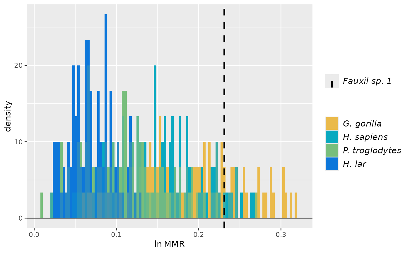
plot(test_faux_uni2, est=2, groupcols=speciescolors)
# Same as above, but variable name information is preserved
test_faux_uni2 <- SSDtest(
fossil=list("Fauxil sp. 1"=fauxil[fauxil$Species=="Fauxil sp. 1", "FHSI", drop=FALSE]),
comp=list("G. gorilla"=apelimbart[apelimbart$Species=="Gorilla gorilla", "FHSI", drop=FALSE],
"H. sapiens"=apelimbart[apelimbart$Species=="Homo sapiens", "FHSI", drop=FALSE],
"P. troglodytes"=apelimbart[apelimbart$Species=="Pan troglodytes","FHSI",drop=FALSE],
"H. lar"=apelimbart[apelimbart$Species=="Hylobates lar", "FHSI", drop=FALSE]),
fossilsex=NULL,
compsex=list("G. gorilla"=apelimbart[apelimbart$Species=="Gorilla gorilla", "Sex"],
"H. sapiens"=apelimbart[apelimbart$Species=="Homo sapiens", "Sex"],
"P. troglodytes"=apelimbart[apelimbart$Species=="Pan troglodytes", "Sex"],
"H. lar"=apelimbart[apelimbart$Species=="Hylobates lar", "Sex"]),
methsUni=c("SSD", "MMR", "BDI"),
limit=1000,
nResamp=100)
#> Warning: The number of possible combinations (3049501) exceeds the user-specified limit. Monte Carlo sampling will be used.
#> Warning: The number of possible combinations (3049501) exceeds the user-specified limit. Monte Carlo sampling will be used.
#> Warning: The number of possible combinations (3049501) exceeds the user-specified limit. Monte Carlo sampling will be used.
#> Warning: The number of possible combinations (3049501) exceeds the user-specified limit. Monte Carlo sampling will be used.
#> Warning: The following comparisons contain NAs that were
#> dropped in the calculation of p-values:
#> SSD:geomean: G. gorilla - H. sapiens
#> SSD:geomean: G. gorilla - P. troglodytes
#> SSD:geomean: G. gorilla - H. lar
#> SSD:geomean: H. sapiens - P. troglodytes
#> SSD:geomean: H. sapiens - H. lar
#> SSD:geomean: P. troglodytes - H. lar
#> SSD:geomean: H. sapiens - G. gorilla
#> SSD:geomean: P. troglodytes - G. gorilla
#> SSD:geomean: H. lar - G. gorilla
#> SSD:geomean: P. troglodytes - H. sapiens
#> SSD:geomean: H. lar - H. sapiens
#> SSD:geomean: H. lar - P. troglodytes
test_faux_uni2
#> SSDtest Object
#>
#> Comparative data set:
#> sample n female n male n unspecified
#> Fauxil sp. 1 0 0 4
#> G. gorilla 47 47 0
#> H. sapiens 47 47 0
#> P. troglodytes 47 47 0
#> H. lar 47 47 0
#> number of variables: 1
#> variable names: FHSI
#> SSD estimate methods (univariate):
#> SSD, MMR, BDI
#> Centering algorithms:
#> geometric mean
#> Number of unique combinations of univariate method and centering algorithm: 3
#>
#> Resampling data structure:
#> sample n resampled data sets resampling type sampling
#> Fauxil sp. 1 1 exact without replacement
#> G. gorilla 100 Monte Carlo without replacement
#> H. sapiens 100 Monte Carlo without replacement
#> P. troglodytes 100 Monte Carlo without replacement
#> H. lar 100 Monte Carlo without replacement
#> number of individuals in each resampled data set: 4
#> other resampling parameters:
#> ratio variables (if present): natural log of ratio
#> matchvars = FALSE
#> na.rm = TRUE
#>
#> Median resampled estimates for each combination of methods:
#> methodUni center Fauxil sp. 1 G. gorilla H. sapiens P. troglodytes H. lar
#> 1 SSD geomean NA 0.1954 0.1511 0.0651 0.0408
#> 2 MMR geomean 0.2312 0.1904 0.1451 0.1083 0.0757
#> 3 BDI geomean 0.1793 0.1590 0.1291 0.0912 0.0650
#>
#> p-values (one-sided; null: first sample less or equally dimorphic as second sample):
#> SSD:geomean MMR:geomean BDI:geomean
#> Fauxil sp. 1 - G. gorilla NA 0.2800 0.4100
#> Fauxil sp. 1 - H. sapiens NA 0.1000 0.1600
#> Fauxil sp. 1 - P. troglodytes NA 0.0200 0.0200
#> Fauxil sp. 1 - H. lar NA 0.0000 0.0000
#> G. gorilla - H. sapiens 0.2782 0.2985 0.3160
#> G. gorilla - P. troglodytes 0.0528 0.1312 0.1520
#> G. gorilla - H. lar 0.0022 0.0201 0.0256
#> H. sapiens - P. troglodytes 0.1530 0.2985 0.2963
#> H. sapiens - H. lar 0.0555 0.1234 0.0887
#> P. troglodytes - H. lar 0.3736 0.2531 0.2080
#> G. gorilla - Fauxil sp. 1 NA 0.7200 0.5900
#> H. sapiens - Fauxil sp. 1 NA 0.9000 0.8400
#> P. troglodytes - Fauxil sp. 1 NA 0.9800 0.9800
#> H. lar - Fauxil sp. 1 NA 1.0000 1.0000
#> H. sapiens - G. gorilla 0.7218 0.7015 0.6840
#> P. troglodytes - G. gorilla 0.9472 0.8688 0.8480
#> H. lar - G. gorilla 0.9978 0.9799 0.9744
#> P. troglodytes - H. sapiens 0.8470 0.7015 0.7037
#> H. lar - H. sapiens 0.9445 0.8766 0.9113
#> H. lar - P. troglodytes 0.6264 0.7469 0.7920
#>
#> p-values (two-sided):
#> SSD:geomean MMR:geomean BDI:geomean
#> Fauxil sp. 1 - G. gorilla NA 0.6000 0.8700
#> Fauxil sp. 1 - H. sapiens NA 0.1900 0.3200
#> Fauxil sp. 1 - P. troglodytes NA 0.0200 0.0200
#> Fauxil sp. 1 - H. lar NA 0.0000 0.0000
#> G. gorilla - H. sapiens 0.5539 0.5954 0.6348
#> G. gorilla - P. troglodytes 0.1207 0.2711 0.3141
#> G. gorilla - H. lar 0.0127 0.0616 0.0535
#> H. sapiens - P. troglodytes 0.3165 0.5925 0.5926
#> H. sapiens - H. lar 0.1151 0.2524 0.1952
#> P. troglodytes - H. lar 0.7859 0.4775 0.4114
#>
#> Warning: The following comparisons contain NAs that were
#> dropped in the calculation of p-values:
#> SSD:geomean: G. gorilla - H. sapiens
#> SSD:geomean: G. gorilla - P. troglodytes
#> SSD:geomean: G. gorilla - H. lar
#> SSD:geomean: H. sapiens - P. troglodytes
#> SSD:geomean: H. sapiens - H. lar
#> SSD:geomean: P. troglodytes - H. lar
#> SSD:geomean: H. sapiens - G. gorilla
#> SSD:geomean: P. troglodytes - G. gorilla
#> SSD:geomean: H. lar - G. gorilla
#> SSD:geomean: P. troglodytes - H. sapiens
#> SSD:geomean: H. lar - H. sapiens
#> SSD:geomean: H. lar - P. troglodytes
plot(test_faux_uni2, est=2, groupcols=speciescolors)
 # Same as above except that null distributions are generated WITH replacement rather than WITHOUT
test_faux_uni3 <- SSDtest(
fossil=list("Fauxil sp. 1"=fauxil[fauxil$Species=="Fauxil sp. 1", "FHSI", drop=FALSE]),
comp=list("G. gorilla"=apelimbart[apelimbart$Species=="Gorilla gorilla", "FHSI", drop=FALSE],
"H. sapiens"=apelimbart[apelimbart$Species=="Homo sapiens", "FHSI", drop=FALSE],
"P. troglodytes"=apelimbart[apelimbart$Species=="Pan troglodytes","FHSI",drop=FALSE],
"H. lar"=apelimbart[apelimbart$Species=="Hylobates lar", "FHSI", drop=FALSE]),
fossilsex=NULL,
compsex=list("G. gorilla"=apelimbart[apelimbart$Species=="Gorilla gorilla", "Sex"],
"H. sapiens"=apelimbart[apelimbart$Species=="Homo sapiens", "Sex"],
"P. troglodytes"=apelimbart[apelimbart$Species=="Pan troglodytes", "Sex"],
"H. lar"=apelimbart[apelimbart$Species=="Hylobates lar", "Sex"]),
methsUni=c("SSD", "MMR", "BDI"),
limit=1000,
nResamp=100,
replace=TRUE)
#> Warning: The number of possible combinations (3464840) exceeds the user-specified limit. Monte Carlo sampling will be used.
#> Warning: The number of possible combinations (3464840) exceeds the user-specified limit. Monte Carlo sampling will be used.
#> Warning: The number of possible combinations (3464840) exceeds the user-specified limit. Monte Carlo sampling will be used.
#> Warning: The number of possible combinations (3464840) exceeds the user-specified limit. Monte Carlo sampling will be used.
#> Warning: The following comparisons contain NAs that were
#> dropped in the calculation of p-values:
#> SSD:geomean: G. gorilla - H. sapiens
#> SSD:geomean: G. gorilla - P. troglodytes
#> SSD:geomean: G. gorilla - H. lar
#> SSD:geomean: H. sapiens - P. troglodytes
#> SSD:geomean: H. sapiens - H. lar
#> SSD:geomean: P. troglodytes - H. lar
#> SSD:geomean: H. sapiens - G. gorilla
#> SSD:geomean: P. troglodytes - G. gorilla
#> SSD:geomean: H. lar - G. gorilla
#> SSD:geomean: P. troglodytes - H. sapiens
#> SSD:geomean: H. lar - H. sapiens
#> SSD:geomean: H. lar - P. troglodytes
test_faux_uni3
#> SSDtest Object
#>
#> Comparative data set:
#> sample n female n male n unspecified
#> Fauxil sp. 1 0 0 4
#> G. gorilla 47 47 0
#> H. sapiens 47 47 0
#> P. troglodytes 47 47 0
#> H. lar 47 47 0
#> number of variables: 1
#> variable names: FHSI
#> SSD estimate methods (univariate):
#> SSD, MMR, BDI
#> Centering algorithms:
#> geometric mean
#> Number of unique combinations of univariate method and centering algorithm: 3
#>
#> Resampling data structure:
#> sample n resampled data sets resampling type sampling
#> Fauxil sp. 1 1 exact without replacement
#> G. gorilla 100 Monte Carlo with replacement
#> H. sapiens 100 Monte Carlo with replacement
#> P. troglodytes 100 Monte Carlo with replacement
#> H. lar 100 Monte Carlo with replacement
#> number of individuals in each resampled data set: 4
#> other resampling parameters:
#> ratio variables (if present): natural log of ratio
#> matchvars = FALSE
#> na.rm = TRUE
#>
#> Median resampled estimates for each combination of methods:
#> methodUni center Fauxil sp. 1 G. gorilla H. sapiens P. troglodytes H. lar
#> 1 SSD geomean NA 0.2012 0.1555 0.0687 0.0223
#> 2 MMR geomean 0.2312 0.1867 0.1544 0.1091 0.0660
#> 3 BDI geomean 0.1793 0.1609 0.1320 0.0993 0.0606
#>
#> p-values (one-sided; null: first sample less or equally dimorphic as second sample):
#> SSD:geomean MMR:geomean BDI:geomean
#> Fauxil sp. 1 - G. gorilla NA 0.2400 0.3600
#> Fauxil sp. 1 - H. sapiens NA 0.0900 0.1500
#> Fauxil sp. 1 - P. troglodytes NA 0.0100 0.0400
#> Fauxil sp. 1 - H. lar NA 0.0000 0.0000
#> G. gorilla - H. sapiens 0.3034 0.3647 0.3405
#> G. gorilla - P. troglodytes 0.0683 0.1862 0.1848
#> G. gorilla - H. lar 0.0053 0.0518 0.0460
#> H. sapiens - P. troglodytes 0.1692 0.2762 0.2958
#> H. sapiens - H. lar 0.0466 0.0836 0.0776
#> P. troglodytes - H. lar 0.2636 0.2211 0.2141
#> G. gorilla - Fauxil sp. 1 NA 0.7600 0.6400
#> H. sapiens - Fauxil sp. 1 NA 0.9100 0.8500
#> P. troglodytes - Fauxil sp. 1 NA 0.9900 0.9600
#> H. lar - Fauxil sp. 1 NA 1.0000 1.0000
#> H. sapiens - G. gorilla 0.6966 0.6353 0.6595
#> P. troglodytes - G. gorilla 0.9317 0.8138 0.8152
#> H. lar - G. gorilla 0.9947 0.9482 0.9540
#> P. troglodytes - H. sapiens 0.8308 0.7238 0.7042
#> H. lar - H. sapiens 0.9534 0.9164 0.9224
#> H. lar - P. troglodytes 0.7364 0.7789 0.7859
#>
#> p-values (two-sided):
#> SSD:geomean MMR:geomean BDI:geomean
#> Fauxil sp. 1 - G. gorilla NA 0.4700 0.7200
#> Fauxil sp. 1 - H. sapiens NA 0.1800 0.2900
#> Fauxil sp. 1 - P. troglodytes NA 0.0100 0.0500
#> Fauxil sp. 1 - H. lar NA 0.0000 0.0000
#> G. gorilla - H. sapiens 0.5941 0.7284 0.6855
#> G. gorilla - P. troglodytes 0.1407 0.3792 0.3734
#> G. gorilla - H. lar 0.0128 0.1059 0.0882
#> H. sapiens - P. troglodytes 0.3372 0.5623 0.5979
#> H. sapiens - H. lar 0.0794 0.1703 0.1591
#> P. troglodytes - H. lar 0.5282 0.4317 0.4207
#>
#> Warning: The following comparisons contain NAs that were
#> dropped in the calculation of p-values:
#> SSD:geomean: G. gorilla - H. sapiens
#> SSD:geomean: G. gorilla - P. troglodytes
#> SSD:geomean: G. gorilla - H. lar
#> SSD:geomean: H. sapiens - P. troglodytes
#> SSD:geomean: H. sapiens - H. lar
#> SSD:geomean: P. troglodytes - H. lar
#> SSD:geomean: H. sapiens - G. gorilla
#> SSD:geomean: P. troglodytes - G. gorilla
#> SSD:geomean: H. lar - G. gorilla
#> SSD:geomean: P. troglodytes - H. sapiens
#> SSD:geomean: H. lar - H. sapiens
#> SSD:geomean: H. lar - P. troglodytes
plot(test_faux_uni3, est=2, groupcols=speciescolors)
# Same as above except that null distributions are generated WITH replacement rather than WITHOUT
test_faux_uni3 <- SSDtest(
fossil=list("Fauxil sp. 1"=fauxil[fauxil$Species=="Fauxil sp. 1", "FHSI", drop=FALSE]),
comp=list("G. gorilla"=apelimbart[apelimbart$Species=="Gorilla gorilla", "FHSI", drop=FALSE],
"H. sapiens"=apelimbart[apelimbart$Species=="Homo sapiens", "FHSI", drop=FALSE],
"P. troglodytes"=apelimbart[apelimbart$Species=="Pan troglodytes","FHSI",drop=FALSE],
"H. lar"=apelimbart[apelimbart$Species=="Hylobates lar", "FHSI", drop=FALSE]),
fossilsex=NULL,
compsex=list("G. gorilla"=apelimbart[apelimbart$Species=="Gorilla gorilla", "Sex"],
"H. sapiens"=apelimbart[apelimbart$Species=="Homo sapiens", "Sex"],
"P. troglodytes"=apelimbart[apelimbart$Species=="Pan troglodytes", "Sex"],
"H. lar"=apelimbart[apelimbart$Species=="Hylobates lar", "Sex"]),
methsUni=c("SSD", "MMR", "BDI"),
limit=1000,
nResamp=100,
replace=TRUE)
#> Warning: The number of possible combinations (3464840) exceeds the user-specified limit. Monte Carlo sampling will be used.
#> Warning: The number of possible combinations (3464840) exceeds the user-specified limit. Monte Carlo sampling will be used.
#> Warning: The number of possible combinations (3464840) exceeds the user-specified limit. Monte Carlo sampling will be used.
#> Warning: The number of possible combinations (3464840) exceeds the user-specified limit. Monte Carlo sampling will be used.
#> Warning: The following comparisons contain NAs that were
#> dropped in the calculation of p-values:
#> SSD:geomean: G. gorilla - H. sapiens
#> SSD:geomean: G. gorilla - P. troglodytes
#> SSD:geomean: G. gorilla - H. lar
#> SSD:geomean: H. sapiens - P. troglodytes
#> SSD:geomean: H. sapiens - H. lar
#> SSD:geomean: P. troglodytes - H. lar
#> SSD:geomean: H. sapiens - G. gorilla
#> SSD:geomean: P. troglodytes - G. gorilla
#> SSD:geomean: H. lar - G. gorilla
#> SSD:geomean: P. troglodytes - H. sapiens
#> SSD:geomean: H. lar - H. sapiens
#> SSD:geomean: H. lar - P. troglodytes
test_faux_uni3
#> SSDtest Object
#>
#> Comparative data set:
#> sample n female n male n unspecified
#> Fauxil sp. 1 0 0 4
#> G. gorilla 47 47 0
#> H. sapiens 47 47 0
#> P. troglodytes 47 47 0
#> H. lar 47 47 0
#> number of variables: 1
#> variable names: FHSI
#> SSD estimate methods (univariate):
#> SSD, MMR, BDI
#> Centering algorithms:
#> geometric mean
#> Number of unique combinations of univariate method and centering algorithm: 3
#>
#> Resampling data structure:
#> sample n resampled data sets resampling type sampling
#> Fauxil sp. 1 1 exact without replacement
#> G. gorilla 100 Monte Carlo with replacement
#> H. sapiens 100 Monte Carlo with replacement
#> P. troglodytes 100 Monte Carlo with replacement
#> H. lar 100 Monte Carlo with replacement
#> number of individuals in each resampled data set: 4
#> other resampling parameters:
#> ratio variables (if present): natural log of ratio
#> matchvars = FALSE
#> na.rm = TRUE
#>
#> Median resampled estimates for each combination of methods:
#> methodUni center Fauxil sp. 1 G. gorilla H. sapiens P. troglodytes H. lar
#> 1 SSD geomean NA 0.2012 0.1555 0.0687 0.0223
#> 2 MMR geomean 0.2312 0.1867 0.1544 0.1091 0.0660
#> 3 BDI geomean 0.1793 0.1609 0.1320 0.0993 0.0606
#>
#> p-values (one-sided; null: first sample less or equally dimorphic as second sample):
#> SSD:geomean MMR:geomean BDI:geomean
#> Fauxil sp. 1 - G. gorilla NA 0.2400 0.3600
#> Fauxil sp. 1 - H. sapiens NA 0.0900 0.1500
#> Fauxil sp. 1 - P. troglodytes NA 0.0100 0.0400
#> Fauxil sp. 1 - H. lar NA 0.0000 0.0000
#> G. gorilla - H. sapiens 0.3034 0.3647 0.3405
#> G. gorilla - P. troglodytes 0.0683 0.1862 0.1848
#> G. gorilla - H. lar 0.0053 0.0518 0.0460
#> H. sapiens - P. troglodytes 0.1692 0.2762 0.2958
#> H. sapiens - H. lar 0.0466 0.0836 0.0776
#> P. troglodytes - H. lar 0.2636 0.2211 0.2141
#> G. gorilla - Fauxil sp. 1 NA 0.7600 0.6400
#> H. sapiens - Fauxil sp. 1 NA 0.9100 0.8500
#> P. troglodytes - Fauxil sp. 1 NA 0.9900 0.9600
#> H. lar - Fauxil sp. 1 NA 1.0000 1.0000
#> H. sapiens - G. gorilla 0.6966 0.6353 0.6595
#> P. troglodytes - G. gorilla 0.9317 0.8138 0.8152
#> H. lar - G. gorilla 0.9947 0.9482 0.9540
#> P. troglodytes - H. sapiens 0.8308 0.7238 0.7042
#> H. lar - H. sapiens 0.9534 0.9164 0.9224
#> H. lar - P. troglodytes 0.7364 0.7789 0.7859
#>
#> p-values (two-sided):
#> SSD:geomean MMR:geomean BDI:geomean
#> Fauxil sp. 1 - G. gorilla NA 0.4700 0.7200
#> Fauxil sp. 1 - H. sapiens NA 0.1800 0.2900
#> Fauxil sp. 1 - P. troglodytes NA 0.0100 0.0500
#> Fauxil sp. 1 - H. lar NA 0.0000 0.0000
#> G. gorilla - H. sapiens 0.5941 0.7284 0.6855
#> G. gorilla - P. troglodytes 0.1407 0.3792 0.3734
#> G. gorilla - H. lar 0.0128 0.1059 0.0882
#> H. sapiens - P. troglodytes 0.3372 0.5623 0.5979
#> H. sapiens - H. lar 0.0794 0.1703 0.1591
#> P. troglodytes - H. lar 0.5282 0.4317 0.4207
#>
#> Warning: The following comparisons contain NAs that were
#> dropped in the calculation of p-values:
#> SSD:geomean: G. gorilla - H. sapiens
#> SSD:geomean: G. gorilla - P. troglodytes
#> SSD:geomean: G. gorilla - H. lar
#> SSD:geomean: H. sapiens - P. troglodytes
#> SSD:geomean: H. sapiens - H. lar
#> SSD:geomean: P. troglodytes - H. lar
#> SSD:geomean: H. sapiens - G. gorilla
#> SSD:geomean: P. troglodytes - G. gorilla
#> SSD:geomean: H. lar - G. gorilla
#> SSD:geomean: P. troglodytes - H. sapiens
#> SSD:geomean: H. lar - H. sapiens
#> SSD:geomean: H. lar - P. troglodytes
plot(test_faux_uni3, est=2, groupcols=speciescolors)
 # Instead of standard test, each comparative and fossil sample is bootstrapped (sampled
# with replacement to that sample's full sample size) by setting 'fullsamplesboot' to
# TRUE. Produces a distribution of fossil estimates rather than a single point estimate,
# but note that comparative samples are resampled to their full sample size, not
# downsampled to the fossil sample size.
test_faux_uni4 <- SSDtest(
fossil=list("Fauxil sp. 1"=fauxil[fauxil$Species=="Fauxil sp. 1", "FHSI", drop=FALSE]),
comp=list("G. gorilla"=apelimbart[apelimbart$Species=="Gorilla gorilla", "FHSI", drop=FALSE],
"H. sapiens"=apelimbart[apelimbart$Species=="Homo sapiens", "FHSI", drop=FALSE],
"P. troglodytes"=apelimbart[apelimbart$Species=="Pan troglodytes","FHSI",drop=FALSE],
"H. lar"=apelimbart[apelimbart$Species=="Hylobates lar", "FHSI", drop=FALSE]),
fossilsex=NULL,
compsex=list("G. gorilla"=apelimbart[apelimbart$Species=="Gorilla gorilla", "Sex"],
"H. sapiens"=apelimbart[apelimbart$Species=="Homo sapiens", "Sex"],
"P. troglodytes"=apelimbart[apelimbart$Species=="Pan troglodytes", "Sex"],
"H. lar"=apelimbart[apelimbart$Species=="Hylobates lar", "Sex"]),
methsUni=c("SSD", "MMR", "BDI"),
limit=1000,
nResamp=100,
fullsamplesboot=TRUE)
#> Warning: The number of possible combinations (1.13996839121089e+55) exceeds the user-specified limit. Monte Carlo sampling will be used.
#> Warning: The number of possible combinations (1.13996839121089e+55) exceeds the user-specified limit. Monte Carlo sampling will be used.
#> Warning: The number of possible combinations (1.13996839121089e+55) exceeds the user-specified limit. Monte Carlo sampling will be used.
#> Warning: The number of possible combinations (1.13996839121089e+55) exceeds the user-specified limit. Monte Carlo sampling will be used.
test_faux_uni4
#> SSDtest Object
#>
#> Comparative data set:
#> sample n female n male n unspecified
#> Fauxil sp. 1 0 0 4
#> G. gorilla 47 47 0
#> H. sapiens 47 47 0
#> P. troglodytes 47 47 0
#> H. lar 47 47 0
#> number of variables: 1
#> variable names: FHSI
#> SSD estimate methods (univariate):
#> SSD, MMR, BDI
#> Centering algorithms:
#> geometric mean
#> Number of unique combinations of univariate method and centering algorithm: 3
#>
#> Resampling data structure:
#> sample n resampled data sets resampling type sampling
#> Fauxil sp. 1 35 exact with replacement
#> G. gorilla 100 Monte Carlo with replacement
#> H. sapiens 100 Monte Carlo with replacement
#> P. troglodytes 100 Monte Carlo with replacement
#> H. lar 100 Monte Carlo with replacement
#> number of individuals in each resampled data set: total sample size within each group
#> resampling procedure:
#> other resampling parameters:
#> ratio variables (if present): natural log of ratio
#> matchvars = FALSE
#> na.rm = TRUE
#>
#> Median resampled estimates for each combination of methods:
#> methodUni center Fauxil sp. 1 G. gorilla H. sapiens P. troglodytes H. lar
#> 1 SSD geomean NA 0.2048 0.1512 0.0670 0.0240
#> 2 MMR geomean 0.1846 0.2054 0.1581 0.1187 0.0767
#> 3 BDI geomean 0.1099 0.2025 0.1549 0.1180 0.0756
#>
#> Two-sided 95% confidence intervals for bootstrapped estimates:
#> methodUni center Fauxil sp. 1 G. gorilla H. sapiens
#> SSD:geomean SSD geomean <NA> 0.1829 to 0.222 0.1298 to 0.1738
#> MMR:geomean MMR geomean 0 to 0.2884 0.1817 to 0.222 0.1387 to 0.1791
#> BDI:geomean BDI geomean 0 to 0.2334 0.1794 to 0.2183 0.1344 to 0.1781
#> P. troglodytes H. lar
#> SSD:geomean 0.0379 to 0.0857 0.0053 to 0.0421
#> MMR:geomean 0.1036 to 0.1404 0.0687 to 0.0876
#> BDI:geomean 0.1039 to 0.1393 0.0684 to 0.0853
#>
#> p-values (one-sided; null: first sample less or equally dimorphic as second sample):
#> SSD:geomean MMR:geomean BDI:geomean
#> Fauxil sp. 1 - G. gorilla NA 0.6180 0.9103
#> Fauxil sp. 1 - H. sapiens NA 0.4571 0.6577
#> Fauxil sp. 1 - P. troglodytes NA 0.4546 0.5134
#> Fauxil sp. 1 - H. lar NA 0.3186 0.4126
#> G. gorilla - H. sapiens 0.0002 0.0007 0.0008
#> G. gorilla - P. troglodytes 0.0000 0.0000 0.0000
#> G. gorilla - H. lar 0.0000 0.0000 0.0000
#> H. sapiens - P. troglodytes 0.0000 0.0014 0.0024
#> H. sapiens - H. lar 0.0000 0.0000 0.0000
#> P. troglodytes - H. lar 0.0026 0.0000 0.0000
#> G. gorilla - Fauxil sp. 1 NA 0.3820 0.0897
#> H. sapiens - Fauxil sp. 1 NA 0.5429 0.3423
#> P. troglodytes - Fauxil sp. 1 NA 0.5454 0.4866
#> H. lar - Fauxil sp. 1 NA 0.6814 0.5874
#> H. sapiens - G. gorilla 0.9998 0.9993 0.9992
#> P. troglodytes - G. gorilla 1.0000 1.0000 1.0000
#> H. lar - G. gorilla 1.0000 1.0000 1.0000
#> P. troglodytes - H. sapiens 1.0000 0.9986 0.9976
#> H. lar - H. sapiens 1.0000 1.0000 1.0000
#> H. lar - P. troglodytes 0.9974 1.0000 1.0000
#>
#> p-values (two-sided):
#> SSD:geomean MMR:geomean BDI:geomean
#> Fauxil sp. 1 - G. gorilla NA 0.7477 0.2086
#> Fauxil sp. 1 - H. sapiens NA 1.0000 0.6660
#> Fauxil sp. 1 - P. troglodytes NA 0.9811 0.9469
#> Fauxil sp. 1 - H. lar NA 0.6109 0.7949
#> G. gorilla - H. sapiens 0.0003 0.0011 0.0011
#> G. gorilla - P. troglodytes 0.0000 0.0000 0.0000
#> G. gorilla - H. lar 0.0000 0.0000 0.0000
#> H. sapiens - P. troglodytes 0.0000 0.0027 0.0047
#> H. sapiens - H. lar 0.0000 0.0000 0.0000
#> P. troglodytes - H. lar 0.0034 0.0000 0.0000
plot(test_faux_uni4, est=2, # plots the second estimation method (MMR)
invert=1, # inverts the histogram for the first group in 'test_afar_uni4'
groupcols=speciescolors)
# Instead of standard test, each comparative and fossil sample is bootstrapped (sampled
# with replacement to that sample's full sample size) by setting 'fullsamplesboot' to
# TRUE. Produces a distribution of fossil estimates rather than a single point estimate,
# but note that comparative samples are resampled to their full sample size, not
# downsampled to the fossil sample size.
test_faux_uni4 <- SSDtest(
fossil=list("Fauxil sp. 1"=fauxil[fauxil$Species=="Fauxil sp. 1", "FHSI", drop=FALSE]),
comp=list("G. gorilla"=apelimbart[apelimbart$Species=="Gorilla gorilla", "FHSI", drop=FALSE],
"H. sapiens"=apelimbart[apelimbart$Species=="Homo sapiens", "FHSI", drop=FALSE],
"P. troglodytes"=apelimbart[apelimbart$Species=="Pan troglodytes","FHSI",drop=FALSE],
"H. lar"=apelimbart[apelimbart$Species=="Hylobates lar", "FHSI", drop=FALSE]),
fossilsex=NULL,
compsex=list("G. gorilla"=apelimbart[apelimbart$Species=="Gorilla gorilla", "Sex"],
"H. sapiens"=apelimbart[apelimbart$Species=="Homo sapiens", "Sex"],
"P. troglodytes"=apelimbart[apelimbart$Species=="Pan troglodytes", "Sex"],
"H. lar"=apelimbart[apelimbart$Species=="Hylobates lar", "Sex"]),
methsUni=c("SSD", "MMR", "BDI"),
limit=1000,
nResamp=100,
fullsamplesboot=TRUE)
#> Warning: The number of possible combinations (1.13996839121089e+55) exceeds the user-specified limit. Monte Carlo sampling will be used.
#> Warning: The number of possible combinations (1.13996839121089e+55) exceeds the user-specified limit. Monte Carlo sampling will be used.
#> Warning: The number of possible combinations (1.13996839121089e+55) exceeds the user-specified limit. Monte Carlo sampling will be used.
#> Warning: The number of possible combinations (1.13996839121089e+55) exceeds the user-specified limit. Monte Carlo sampling will be used.
test_faux_uni4
#> SSDtest Object
#>
#> Comparative data set:
#> sample n female n male n unspecified
#> Fauxil sp. 1 0 0 4
#> G. gorilla 47 47 0
#> H. sapiens 47 47 0
#> P. troglodytes 47 47 0
#> H. lar 47 47 0
#> number of variables: 1
#> variable names: FHSI
#> SSD estimate methods (univariate):
#> SSD, MMR, BDI
#> Centering algorithms:
#> geometric mean
#> Number of unique combinations of univariate method and centering algorithm: 3
#>
#> Resampling data structure:
#> sample n resampled data sets resampling type sampling
#> Fauxil sp. 1 35 exact with replacement
#> G. gorilla 100 Monte Carlo with replacement
#> H. sapiens 100 Monte Carlo with replacement
#> P. troglodytes 100 Monte Carlo with replacement
#> H. lar 100 Monte Carlo with replacement
#> number of individuals in each resampled data set: total sample size within each group
#> resampling procedure:
#> other resampling parameters:
#> ratio variables (if present): natural log of ratio
#> matchvars = FALSE
#> na.rm = TRUE
#>
#> Median resampled estimates for each combination of methods:
#> methodUni center Fauxil sp. 1 G. gorilla H. sapiens P. troglodytes H. lar
#> 1 SSD geomean NA 0.2048 0.1512 0.0670 0.0240
#> 2 MMR geomean 0.1846 0.2054 0.1581 0.1187 0.0767
#> 3 BDI geomean 0.1099 0.2025 0.1549 0.1180 0.0756
#>
#> Two-sided 95% confidence intervals for bootstrapped estimates:
#> methodUni center Fauxil sp. 1 G. gorilla H. sapiens
#> SSD:geomean SSD geomean <NA> 0.1829 to 0.222 0.1298 to 0.1738
#> MMR:geomean MMR geomean 0 to 0.2884 0.1817 to 0.222 0.1387 to 0.1791
#> BDI:geomean BDI geomean 0 to 0.2334 0.1794 to 0.2183 0.1344 to 0.1781
#> P. troglodytes H. lar
#> SSD:geomean 0.0379 to 0.0857 0.0053 to 0.0421
#> MMR:geomean 0.1036 to 0.1404 0.0687 to 0.0876
#> BDI:geomean 0.1039 to 0.1393 0.0684 to 0.0853
#>
#> p-values (one-sided; null: first sample less or equally dimorphic as second sample):
#> SSD:geomean MMR:geomean BDI:geomean
#> Fauxil sp. 1 - G. gorilla NA 0.6180 0.9103
#> Fauxil sp. 1 - H. sapiens NA 0.4571 0.6577
#> Fauxil sp. 1 - P. troglodytes NA 0.4546 0.5134
#> Fauxil sp. 1 - H. lar NA 0.3186 0.4126
#> G. gorilla - H. sapiens 0.0002 0.0007 0.0008
#> G. gorilla - P. troglodytes 0.0000 0.0000 0.0000
#> G. gorilla - H. lar 0.0000 0.0000 0.0000
#> H. sapiens - P. troglodytes 0.0000 0.0014 0.0024
#> H. sapiens - H. lar 0.0000 0.0000 0.0000
#> P. troglodytes - H. lar 0.0026 0.0000 0.0000
#> G. gorilla - Fauxil sp. 1 NA 0.3820 0.0897
#> H. sapiens - Fauxil sp. 1 NA 0.5429 0.3423
#> P. troglodytes - Fauxil sp. 1 NA 0.5454 0.4866
#> H. lar - Fauxil sp. 1 NA 0.6814 0.5874
#> H. sapiens - G. gorilla 0.9998 0.9993 0.9992
#> P. troglodytes - G. gorilla 1.0000 1.0000 1.0000
#> H. lar - G. gorilla 1.0000 1.0000 1.0000
#> P. troglodytes - H. sapiens 1.0000 0.9986 0.9976
#> H. lar - H. sapiens 1.0000 1.0000 1.0000
#> H. lar - P. troglodytes 0.9974 1.0000 1.0000
#>
#> p-values (two-sided):
#> SSD:geomean MMR:geomean BDI:geomean
#> Fauxil sp. 1 - G. gorilla NA 0.7477 0.2086
#> Fauxil sp. 1 - H. sapiens NA 1.0000 0.6660
#> Fauxil sp. 1 - P. troglodytes NA 0.9811 0.9469
#> Fauxil sp. 1 - H. lar NA 0.6109 0.7949
#> G. gorilla - H. sapiens 0.0003 0.0011 0.0011
#> G. gorilla - P. troglodytes 0.0000 0.0000 0.0000
#> G. gorilla - H. lar 0.0000 0.0000 0.0000
#> H. sapiens - P. troglodytes 0.0000 0.0027 0.0047
#> H. sapiens - H. lar 0.0000 0.0000 0.0000
#> P. troglodytes - H. lar 0.0034 0.0000 0.0000
plot(test_faux_uni4, est=2, # plots the second estimation method (MMR)
invert=1, # inverts the histogram for the first group in 'test_afar_uni4'
groupcols=speciescolors)
 ## Multivariate examples
# GMM significance tests with a fossil sample for multiple estimators using both complete
# and incomplete comparative datasets. A single point estimate is generated for the fossil
# sample for each method.
SSDvars <- c("FHSI", "TPML", "TPMAP", "TPLAP", "HHMaj",
"HHMin", "RHMaj", "RHMin", "RDAP", "RDML")
test_faux_multi1 <- SSDtest(
fossil=list("Fauxil sp. 1"=fauxil[fauxil$Species=="Fauxil sp. 1", SSDvars]),
comp=list("G. gorilla"=apelimbart[apelimbart$Species=="Gorilla gorilla", SSDvars],
"H. sapiens"=apelimbart[apelimbart$Species=="Homo sapiens", SSDvars],
"P. troglodytes"=apelimbart[apelimbart$Species=="Pan troglodytes", SSDvars],
"H. lar"=apelimbart[apelimbart$Species=="Hylobates lar", SSDvars]),
fossilsex=NULL,
compsex=list("G. gorilla"=apelimbart[apelimbart$Species=="Gorilla gorilla", "Sex"],
"H. sapiens"=apelimbart[apelimbart$Species=="Homo sapiens", "Sex"],
"P. troglodytes"=apelimbart[apelimbart$Species=="Pan troglodytes", "Sex"],
"H. lar"=apelimbart[apelimbart$Species=="Hylobates lar", "Sex"]),
methsUni=c("MMR", "BDI"),
methsMulti=c("GMM"),
datastruc="both",
nResamp=100)
#> Warning: The number of possible combinations (9.60207663113656e+30) exceeds the user-specified limit. Monte Carlo sampling will be used.
#> Warning: The number of possible combinations (9.60207663113656e+30) exceeds the user-specified limit. Monte Carlo sampling will be used.
#> Warning: The number of possible combinations (9.60207663113656e+30) exceeds the user-specified limit. Monte Carlo sampling will be used.
#> Warning: The number of possible combinations (9.60207663113656e+30) exceeds the user-specified limit. Monte Carlo sampling will be used.
test_faux_multi1
#> SSDtest Object
#>
#> Comparative data set:
#> sample n female n male n unspecified
#> Fauxil sp. 1 0 0 16
#> G. gorilla 47 47 0
#> H. sapiens 47 47 0
#> P. troglodytes 47 47 0
#> H. lar 47 47 0
#> number of variables: 10
#> variable names: FHSI, TPML, TPMAP, TPLAP, HHMaj, HHMin, RHMaj, RHMin, RDAP, RDML
#> SSD estimate methods (univariate):
#> MMR, BDI
#> SSD estimate methods (multivariate):
#> GMM
#> Centering algorithms:
#> geometric mean
#> Multivariate sampling with complete or missing data:
#> complete and missing
#> Number of unique combinations of univariate method, multivariate method,
#> centering algorithm, and complete or missing data structure: 4
#>
#> Resampling data structure:
#> sample n resampled data sets resampling type sampling
#> Fauxil sp. 1 1 exact without replacement
#> G. gorilla 100 Monte Carlo without replacement
#> H. sapiens 100 Monte Carlo without replacement
#> P. troglodytes 100 Monte Carlo without replacement
#> H. lar 100 Monte Carlo without replacement
#> missing data resampling structure:
#> sampling individuals, then imposing missing data pattern
#> number of individuals in each resampled data set: 16
#> proportion of missing data in resampling structure: 0.775
#> other resampling parameters:
#> ratio variables (if present): natural log of ratio
#> matchvars = FALSE
#> na.rm = TRUE
#>
#> Median resampled estimates for each combination of methods:
#> methodUni methodMulti center datastructure Fauxil sp. 1 G. gorilla
#> 1 MMR GMM geomean complete NA 0.2226
#> 2 MMR GMM geomean missing 0.2251 0.1874
#> 3 BDI GMM geomean complete NA 0.2097
#> 4 BDI GMM geomean missing 0.2007 0.1645
#> H. sapiens P. troglodytes H. lar
#> 1 0.1552 0.1205 0.0849
#> 2 0.1323 0.1062 0.0730
#> 3 0.1490 0.1175 0.0827
#> 4 0.1208 0.0966 0.0681
#>
#> p-values (one-sided; null: first sample less or equally dimorphic as second sample):
#> MMR:GMM:geomean:complete MMR:GMM:geomean:missing
#> Fauxil sp. 1 - G. gorilla NA 0.1200
#> Fauxil sp. 1 - H. sapiens NA 0.0000
#> Fauxil sp. 1 - P. troglodytes NA 0.0000
#> Fauxil sp. 1 - H. lar NA 0.0000
#> G. gorilla - H. sapiens 0.0071 0.0963
#> G. gorilla - P. troglodytes 0.0000 0.0171
#> G. gorilla - H. lar 0.0000 0.0000
#> H. sapiens - P. troglodytes 0.0696 0.2147
#> H. sapiens - H. lar 0.0000 0.0129
#> P. troglodytes - H. lar 0.0127 0.0783
#> G. gorilla - Fauxil sp. 1 NA 0.8800
#> H. sapiens - Fauxil sp. 1 NA 1.0000
#> P. troglodytes - Fauxil sp. 1 NA 1.0000
#> H. lar - Fauxil sp. 1 NA 1.0000
#> H. sapiens - G. gorilla 0.9929 0.9037
#> P. troglodytes - G. gorilla 1.0000 0.9829
#> H. lar - G. gorilla 1.0000 1.0000
#> P. troglodytes - H. sapiens 0.9304 0.7853
#> H. lar - H. sapiens 1.0000 0.9871
#> H. lar - P. troglodytes 0.9873 0.9217
#> BDI:GMM:geomean:complete BDI:GMM:geomean:missing
#> Fauxil sp. 1 - G. gorilla NA 0.1400
#> Fauxil sp. 1 - H. sapiens NA 0.0000
#> Fauxil sp. 1 - P. troglodytes NA 0.0000
#> Fauxil sp. 1 - H. lar NA 0.0000
#> G. gorilla - H. sapiens 0.0098 0.1036
#> G. gorilla - P. troglodytes 0.0000 0.0187
#> G. gorilla - H. lar 0.0000 0.0000
#> H. sapiens - P. troglodytes 0.0755 0.2210
#> H. sapiens - H. lar 0.0000 0.0119
#> P. troglodytes - H. lar 0.0099 0.0791
#> G. gorilla - Fauxil sp. 1 NA 0.8600
#> H. sapiens - Fauxil sp. 1 NA 1.0000
#> P. troglodytes - Fauxil sp. 1 NA 1.0000
#> H. lar - Fauxil sp. 1 NA 1.0000
#> H. sapiens - G. gorilla 0.9902 0.8964
#> P. troglodytes - G. gorilla 1.0000 0.9813
#> H. lar - G. gorilla 1.0000 1.0000
#> P. troglodytes - H. sapiens 0.9245 0.7790
#> H. lar - H. sapiens 1.0000 0.9881
#> H. lar - P. troglodytes 0.9901 0.9209
#>
#> p-values (two-sided):
#> MMR:GMM:geomean:complete MMR:GMM:geomean:missing
#> Fauxil sp. 1 - G. gorilla NA 0.2800
#> Fauxil sp. 1 - H. sapiens NA 0.0000
#> Fauxil sp. 1 - P. troglodytes NA 0.0000
#> Fauxil sp. 1 - H. lar NA 0.0000
#> G. gorilla - H. sapiens 0.0156 0.1963
#> G. gorilla - P. troglodytes 0.0000 0.0433
#> G. gorilla - H. lar 0.0000 0.0024
#> H. sapiens - P. troglodytes 0.1362 0.4317
#> H. sapiens - H. lar 0.0000 0.0272
#> P. troglodytes - H. lar 0.0317 0.1706
#> BDI:GMM:geomean:complete BDI:GMM:geomean:missing
#> Fauxil sp. 1 - G. gorilla NA 0.2900
#> Fauxil sp. 1 - H. sapiens NA 0.0000
#> Fauxil sp. 1 - P. troglodytes NA 0.0000
#> Fauxil sp. 1 - H. lar NA 0.0000
#> G. gorilla - H. sapiens 0.0201 0.2123
#> G. gorilla - P. troglodytes 0.0000 0.0473
#> G. gorilla - H. lar 0.0000 0.0045
#> H. sapiens - P. troglodytes 0.1472 0.4496
#> H. sapiens - H. lar 0.0002 0.0235
#> P. troglodytes - H. lar 0.0273 0.1740
plot(test_faux_multi1, groupcols=speciescolors)
## Multivariate examples
# GMM significance tests with a fossil sample for multiple estimators using both complete
# and incomplete comparative datasets. A single point estimate is generated for the fossil
# sample for each method.
SSDvars <- c("FHSI", "TPML", "TPMAP", "TPLAP", "HHMaj",
"HHMin", "RHMaj", "RHMin", "RDAP", "RDML")
test_faux_multi1 <- SSDtest(
fossil=list("Fauxil sp. 1"=fauxil[fauxil$Species=="Fauxil sp. 1", SSDvars]),
comp=list("G. gorilla"=apelimbart[apelimbart$Species=="Gorilla gorilla", SSDvars],
"H. sapiens"=apelimbart[apelimbart$Species=="Homo sapiens", SSDvars],
"P. troglodytes"=apelimbart[apelimbart$Species=="Pan troglodytes", SSDvars],
"H. lar"=apelimbart[apelimbart$Species=="Hylobates lar", SSDvars]),
fossilsex=NULL,
compsex=list("G. gorilla"=apelimbart[apelimbart$Species=="Gorilla gorilla", "Sex"],
"H. sapiens"=apelimbart[apelimbart$Species=="Homo sapiens", "Sex"],
"P. troglodytes"=apelimbart[apelimbart$Species=="Pan troglodytes", "Sex"],
"H. lar"=apelimbart[apelimbart$Species=="Hylobates lar", "Sex"]),
methsUni=c("MMR", "BDI"),
methsMulti=c("GMM"),
datastruc="both",
nResamp=100)
#> Warning: The number of possible combinations (9.60207663113656e+30) exceeds the user-specified limit. Monte Carlo sampling will be used.
#> Warning: The number of possible combinations (9.60207663113656e+30) exceeds the user-specified limit. Monte Carlo sampling will be used.
#> Warning: The number of possible combinations (9.60207663113656e+30) exceeds the user-specified limit. Monte Carlo sampling will be used.
#> Warning: The number of possible combinations (9.60207663113656e+30) exceeds the user-specified limit. Monte Carlo sampling will be used.
test_faux_multi1
#> SSDtest Object
#>
#> Comparative data set:
#> sample n female n male n unspecified
#> Fauxil sp. 1 0 0 16
#> G. gorilla 47 47 0
#> H. sapiens 47 47 0
#> P. troglodytes 47 47 0
#> H. lar 47 47 0
#> number of variables: 10
#> variable names: FHSI, TPML, TPMAP, TPLAP, HHMaj, HHMin, RHMaj, RHMin, RDAP, RDML
#> SSD estimate methods (univariate):
#> MMR, BDI
#> SSD estimate methods (multivariate):
#> GMM
#> Centering algorithms:
#> geometric mean
#> Multivariate sampling with complete or missing data:
#> complete and missing
#> Number of unique combinations of univariate method, multivariate method,
#> centering algorithm, and complete or missing data structure: 4
#>
#> Resampling data structure:
#> sample n resampled data sets resampling type sampling
#> Fauxil sp. 1 1 exact without replacement
#> G. gorilla 100 Monte Carlo without replacement
#> H. sapiens 100 Monte Carlo without replacement
#> P. troglodytes 100 Monte Carlo without replacement
#> H. lar 100 Monte Carlo without replacement
#> missing data resampling structure:
#> sampling individuals, then imposing missing data pattern
#> number of individuals in each resampled data set: 16
#> proportion of missing data in resampling structure: 0.775
#> other resampling parameters:
#> ratio variables (if present): natural log of ratio
#> matchvars = FALSE
#> na.rm = TRUE
#>
#> Median resampled estimates for each combination of methods:
#> methodUni methodMulti center datastructure Fauxil sp. 1 G. gorilla
#> 1 MMR GMM geomean complete NA 0.2226
#> 2 MMR GMM geomean missing 0.2251 0.1874
#> 3 BDI GMM geomean complete NA 0.2097
#> 4 BDI GMM geomean missing 0.2007 0.1645
#> H. sapiens P. troglodytes H. lar
#> 1 0.1552 0.1205 0.0849
#> 2 0.1323 0.1062 0.0730
#> 3 0.1490 0.1175 0.0827
#> 4 0.1208 0.0966 0.0681
#>
#> p-values (one-sided; null: first sample less or equally dimorphic as second sample):
#> MMR:GMM:geomean:complete MMR:GMM:geomean:missing
#> Fauxil sp. 1 - G. gorilla NA 0.1200
#> Fauxil sp. 1 - H. sapiens NA 0.0000
#> Fauxil sp. 1 - P. troglodytes NA 0.0000
#> Fauxil sp. 1 - H. lar NA 0.0000
#> G. gorilla - H. sapiens 0.0071 0.0963
#> G. gorilla - P. troglodytes 0.0000 0.0171
#> G. gorilla - H. lar 0.0000 0.0000
#> H. sapiens - P. troglodytes 0.0696 0.2147
#> H. sapiens - H. lar 0.0000 0.0129
#> P. troglodytes - H. lar 0.0127 0.0783
#> G. gorilla - Fauxil sp. 1 NA 0.8800
#> H. sapiens - Fauxil sp. 1 NA 1.0000
#> P. troglodytes - Fauxil sp. 1 NA 1.0000
#> H. lar - Fauxil sp. 1 NA 1.0000
#> H. sapiens - G. gorilla 0.9929 0.9037
#> P. troglodytes - G. gorilla 1.0000 0.9829
#> H. lar - G. gorilla 1.0000 1.0000
#> P. troglodytes - H. sapiens 0.9304 0.7853
#> H. lar - H. sapiens 1.0000 0.9871
#> H. lar - P. troglodytes 0.9873 0.9217
#> BDI:GMM:geomean:complete BDI:GMM:geomean:missing
#> Fauxil sp. 1 - G. gorilla NA 0.1400
#> Fauxil sp. 1 - H. sapiens NA 0.0000
#> Fauxil sp. 1 - P. troglodytes NA 0.0000
#> Fauxil sp. 1 - H. lar NA 0.0000
#> G. gorilla - H. sapiens 0.0098 0.1036
#> G. gorilla - P. troglodytes 0.0000 0.0187
#> G. gorilla - H. lar 0.0000 0.0000
#> H. sapiens - P. troglodytes 0.0755 0.2210
#> H. sapiens - H. lar 0.0000 0.0119
#> P. troglodytes - H. lar 0.0099 0.0791
#> G. gorilla - Fauxil sp. 1 NA 0.8600
#> H. sapiens - Fauxil sp. 1 NA 1.0000
#> P. troglodytes - Fauxil sp. 1 NA 1.0000
#> H. lar - Fauxil sp. 1 NA 1.0000
#> H. sapiens - G. gorilla 0.9902 0.8964
#> P. troglodytes - G. gorilla 1.0000 0.9813
#> H. lar - G. gorilla 1.0000 1.0000
#> P. troglodytes - H. sapiens 0.9245 0.7790
#> H. lar - H. sapiens 1.0000 0.9881
#> H. lar - P. troglodytes 0.9901 0.9209
#>
#> p-values (two-sided):
#> MMR:GMM:geomean:complete MMR:GMM:geomean:missing
#> Fauxil sp. 1 - G. gorilla NA 0.2800
#> Fauxil sp. 1 - H. sapiens NA 0.0000
#> Fauxil sp. 1 - P. troglodytes NA 0.0000
#> Fauxil sp. 1 - H. lar NA 0.0000
#> G. gorilla - H. sapiens 0.0156 0.1963
#> G. gorilla - P. troglodytes 0.0000 0.0433
#> G. gorilla - H. lar 0.0000 0.0024
#> H. sapiens - P. troglodytes 0.1362 0.4317
#> H. sapiens - H. lar 0.0000 0.0272
#> P. troglodytes - H. lar 0.0317 0.1706
#> BDI:GMM:geomean:complete BDI:GMM:geomean:missing
#> Fauxil sp. 1 - G. gorilla NA 0.2900
#> Fauxil sp. 1 - H. sapiens NA 0.0000
#> Fauxil sp. 1 - P. troglodytes NA 0.0000
#> Fauxil sp. 1 - H. lar NA 0.0000
#> G. gorilla - H. sapiens 0.0201 0.2123
#> G. gorilla - P. troglodytes 0.0000 0.0473
#> G. gorilla - H. lar 0.0000 0.0045
#> H. sapiens - P. troglodytes 0.1472 0.4496
#> H. sapiens - H. lar 0.0002 0.0235
#> P. troglodytes - H. lar 0.0273 0.1740
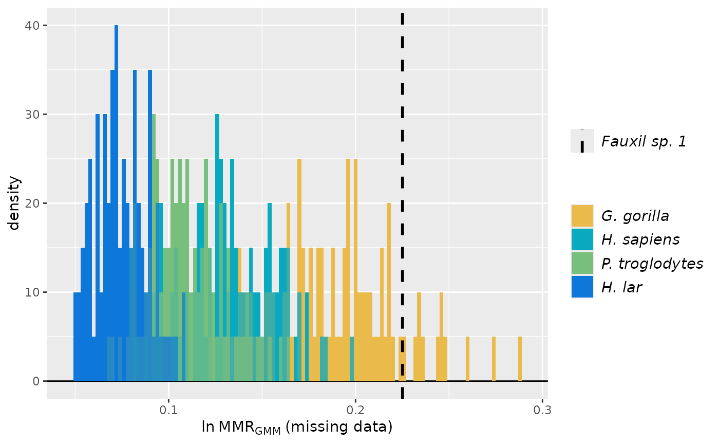
plot(test_faux_multi1, groupcols=speciescolors)
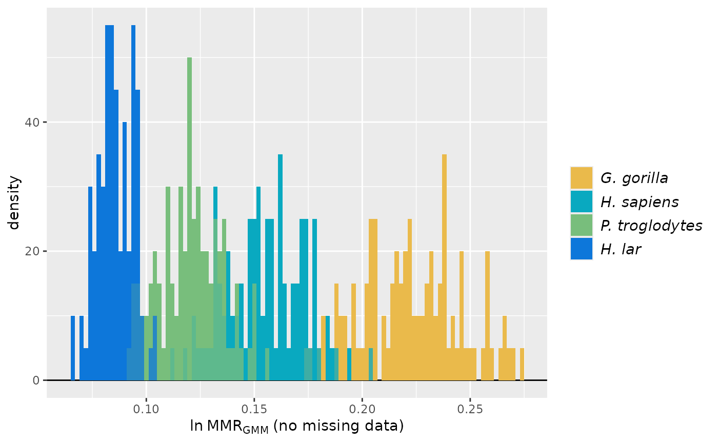 plot(test_faux_multi1, est=2, # plot the 2nd method combination: MMR, GMM, missing datastructure
groupcols=speciescolors)
plot(test_faux_multi1, est=2, # plot the 2nd method combination: MMR, GMM, missing datastructure
groupcols=speciescolors)
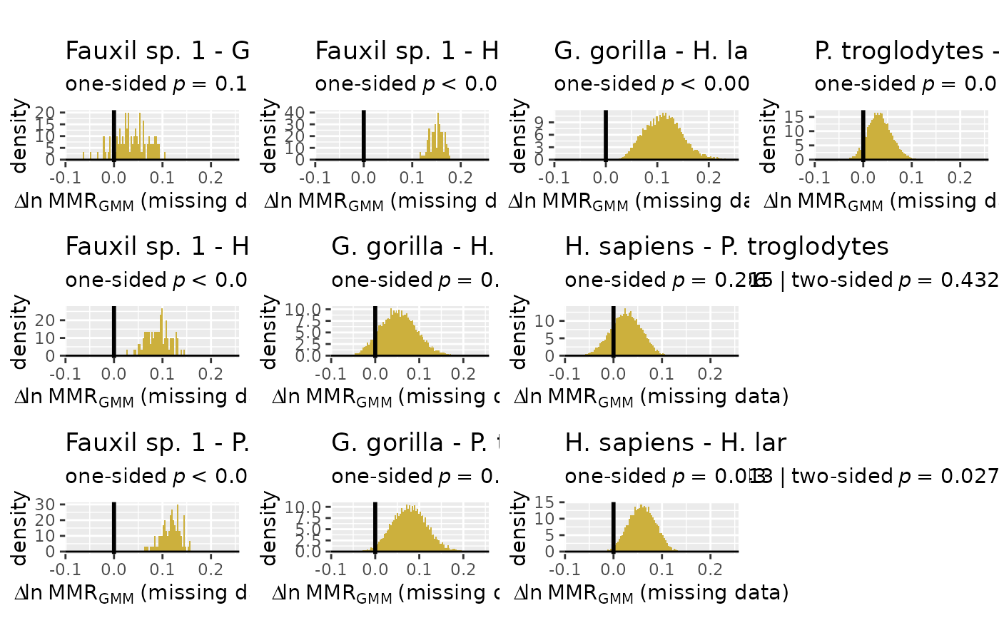
 plot(test_faux_multi1, est=2,
type="diff") # plot the diffs between samples for estimates using the 2nd method combination
plot(test_faux_multi1, est=2,
type="diff") # plot the diffs between samples for estimates using the 2nd method combination
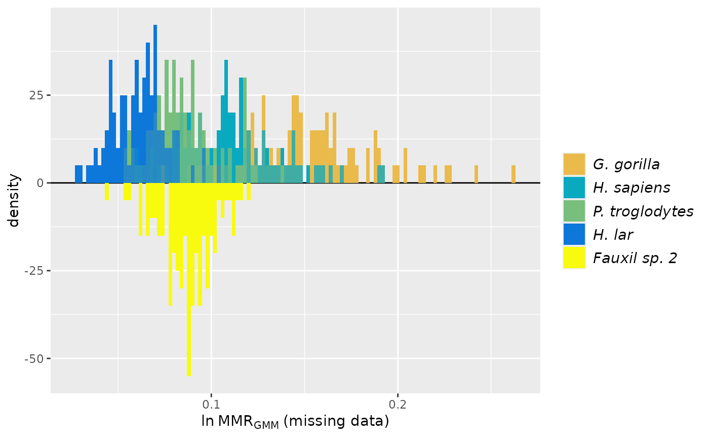
 # As above but with a different fossil sample.
test_faux_multi2 <- SSDtest(
fossil=list("Fauxil sp. 2"=fauxil[fauxil$Species=="Fauxil sp. 2", SSDvars]),
comp=list("G. gorilla"=apelimbart[apelimbart$Species=="Gorilla gorilla", SSDvars],
"H. sapiens"=apelimbart[apelimbart$Species=="Homo sapiens", SSDvars],
"P. troglodytes"=apelimbart[apelimbart$Species=="Pan troglodytes", SSDvars],
"H. lar"=apelimbart[apelimbart$Species=="Hylobates lar", SSDvars]),
fossilsex=NULL,
compsex=list("G. gorilla"=apelimbart[apelimbart$Species=="Gorilla gorilla", "Sex"],
"H. sapiens"=apelimbart[apelimbart$Species=="Homo sapiens", "Sex"],
"P. troglodytes"=apelimbart[apelimbart$Species=="Pan troglodytes", "Sex"],
"H. lar"=apelimbart[apelimbart$Species=="Hylobates lar", "Sex"]),
methsUni=c("MMR", "BDI"),
methsMulti=c("GMM"),
datastruc="both",
nResamp=100)
#> Warning: The number of possible combinations (5.47865686342759e+35) exceeds the user-specified limit. Monte Carlo sampling will be used.
#> Warning: The number of possible combinations (5.47865686342759e+35) exceeds the user-specified limit. Monte Carlo sampling will be used.
#> Warning: The number of possible combinations (5.47865686342759e+35) exceeds the user-specified limit. Monte Carlo sampling will be used.
#> Warning: The number of possible combinations (5.47865686342759e+35) exceeds the user-specified limit. Monte Carlo sampling will be used.
test_faux_multi2
#> SSDtest Object
#>
#> Comparative data set:
#> sample n female n male n unspecified
#> Fauxil sp. 2 0 0 19
#> G. gorilla 47 47 0
#> H. sapiens 47 47 0
#> P. troglodytes 47 47 0
#> H. lar 47 47 0
#> number of variables: 9
#> variable names: FHSI, TPML, TPMAP, TPLAP, HHMaj, HHMin, RHMaj, RDAP, RDML
#> SSD estimate methods (univariate):
#> MMR, BDI
#> SSD estimate methods (multivariate):
#> GMM
#> Centering algorithms:
#> geometric mean
#> Multivariate sampling with complete or missing data:
#> complete and missing
#> Number of unique combinations of univariate method, multivariate method,
#> centering algorithm, and complete or missing data structure: 4
#>
#> Resampling data structure:
#> sample n resampled data sets resampling type sampling
#> Fauxil sp. 2 1 exact without replacement
#> G. gorilla 100 Monte Carlo without replacement
#> H. sapiens 100 Monte Carlo without replacement
#> P. troglodytes 100 Monte Carlo without replacement
#> H. lar 100 Monte Carlo without replacement
#> missing data resampling structure:
#> sampling individuals, then imposing missing data pattern
#> number of individuals in each resampled data set: 19
#> proportion of missing data in resampling structure: 0.784
#> other resampling parameters:
#> ratio variables (if present): natural log of ratio
#> matchvars = FALSE
#> na.rm = TRUE
#>
#> Median resampled estimates for each combination of methods:
#> methodUni methodMulti center datastructure Fauxil sp. 2 G. gorilla
#> 1 MMR GMM geomean complete NA 0.2262
#> 2 MMR GMM geomean missing 0.1072 0.1962
#> 3 BDI GMM geomean complete NA 0.2156
#> 4 BDI GMM geomean missing 0.0966 0.1742
#> H. sapiens P. troglodytes H. lar
#> 1 0.1528 0.1168 0.0836
#> 2 0.1305 0.1012 0.0753
#> 3 0.1491 0.1140 0.0816
#> 4 0.1193 0.0928 0.0694
#>
#> p-values (one-sided; null: first sample less or equally dimorphic as second sample):
#> MMR:GMM:geomean:complete MMR:GMM:geomean:missing
#> Fauxil sp. 2 - G. gorilla NA 1.0000
#> Fauxil sp. 2 - H. sapiens NA 0.8900
#> Fauxil sp. 2 - P. troglodytes NA 0.3800
#> Fauxil sp. 2 - H. lar NA 0.0200
#> G. gorilla - H. sapiens 0.0004 0.0247
#> G. gorilla - P. troglodytes 0.0000 0.0014
#> G. gorilla - H. lar 0.0000 0.0000
#> H. sapiens - P. troglodytes 0.0207 0.1497
#> H. sapiens - H. lar 0.0000 0.0092
#> P. troglodytes - H. lar 0.0041 0.1040
#> G. gorilla - Fauxil sp. 2 NA 0.0000
#> H. sapiens - Fauxil sp. 2 NA 0.1100
#> P. troglodytes - Fauxil sp. 2 NA 0.6200
#> H. lar - Fauxil sp. 2 NA 0.9800
#> H. sapiens - G. gorilla 0.9996 0.9753
#> P. troglodytes - G. gorilla 1.0000 0.9986
#> H. lar - G. gorilla 1.0000 1.0000
#> P. troglodytes - H. sapiens 0.9793 0.8503
#> H. lar - H. sapiens 1.0000 0.9908
#> H. lar - P. troglodytes 0.9959 0.8960
#> BDI:GMM:geomean:complete BDI:GMM:geomean:missing
#> Fauxil sp. 2 - G. gorilla NA 1.0000
#> Fauxil sp. 2 - H. sapiens NA 0.9000
#> Fauxil sp. 2 - P. troglodytes NA 0.4200
#> Fauxil sp. 2 - H. lar NA 0.0100
#> G. gorilla - H. sapiens 0.0006 0.0359
#> G. gorilla - P. troglodytes 0.0000 0.0009
#> G. gorilla - H. lar 0.0000 0.0000
#> H. sapiens - P. troglodytes 0.0241 0.1476
#> H. sapiens - H. lar 0.0000 0.0091
#> P. troglodytes - H. lar 0.0046 0.1137
#> G. gorilla - Fauxil sp. 2 NA 0.0000
#> H. sapiens - Fauxil sp. 2 NA 0.1000
#> P. troglodytes - Fauxil sp. 2 NA 0.5800
#> H. lar - Fauxil sp. 2 NA 0.9900
#> H. sapiens - G. gorilla 0.9994 0.9641
#> P. troglodytes - G. gorilla 1.0000 0.9991
#> H. lar - G. gorilla 1.0000 1.0000
#> P. troglodytes - H. sapiens 0.9759 0.8524
#> H. lar - H. sapiens 1.0000 0.9909
#> H. lar - P. troglodytes 0.9954 0.8863
#>
#> p-values (two-sided):
#> MMR:GMM:geomean:complete MMR:GMM:geomean:missing
#> Fauxil sp. 2 - G. gorilla NA 0.0000
#> Fauxil sp. 2 - H. sapiens NA 0.2200
#> Fauxil sp. 2 - P. troglodytes NA 0.8100
#> Fauxil sp. 2 - H. lar NA 0.0200
#> G. gorilla - H. sapiens 0.0007 0.0467
#> G. gorilla - P. troglodytes 0.0000 0.0029
#> G. gorilla - H. lar 0.0000 0.0000
#> H. sapiens - P. troglodytes 0.0400 0.2991
#> H. sapiens - H. lar 0.0000 0.0215
#> P. troglodytes - H. lar 0.0084 0.2151
#> BDI:GMM:geomean:complete BDI:GMM:geomean:missing
#> Fauxil sp. 2 - G. gorilla NA 0.0000
#> Fauxil sp. 2 - H. sapiens NA 0.2100
#> Fauxil sp. 2 - P. troglodytes NA 0.8600
#> Fauxil sp. 2 - H. lar NA 0.0100
#> G. gorilla - H. sapiens 0.0016 0.0703
#> G. gorilla - P. troglodytes 0.0000 0.0023
#> G. gorilla - H. lar 0.0000 0.0000
#> H. sapiens - P. troglodytes 0.0465 0.2927
#> H. sapiens - H. lar 0.0000 0.0232
#> P. troglodytes - H. lar 0.0076 0.2323
plot(test_faux_multi2, groupcols=speciescolors)
# As above but with a different fossil sample.
test_faux_multi2 <- SSDtest(
fossil=list("Fauxil sp. 2"=fauxil[fauxil$Species=="Fauxil sp. 2", SSDvars]),
comp=list("G. gorilla"=apelimbart[apelimbart$Species=="Gorilla gorilla", SSDvars],
"H. sapiens"=apelimbart[apelimbart$Species=="Homo sapiens", SSDvars],
"P. troglodytes"=apelimbart[apelimbart$Species=="Pan troglodytes", SSDvars],
"H. lar"=apelimbart[apelimbart$Species=="Hylobates lar", SSDvars]),
fossilsex=NULL,
compsex=list("G. gorilla"=apelimbart[apelimbart$Species=="Gorilla gorilla", "Sex"],
"H. sapiens"=apelimbart[apelimbart$Species=="Homo sapiens", "Sex"],
"P. troglodytes"=apelimbart[apelimbart$Species=="Pan troglodytes", "Sex"],
"H. lar"=apelimbart[apelimbart$Species=="Hylobates lar", "Sex"]),
methsUni=c("MMR", "BDI"),
methsMulti=c("GMM"),
datastruc="both",
nResamp=100)
#> Warning: The number of possible combinations (5.47865686342759e+35) exceeds the user-specified limit. Monte Carlo sampling will be used.
#> Warning: The number of possible combinations (5.47865686342759e+35) exceeds the user-specified limit. Monte Carlo sampling will be used.
#> Warning: The number of possible combinations (5.47865686342759e+35) exceeds the user-specified limit. Monte Carlo sampling will be used.
#> Warning: The number of possible combinations (5.47865686342759e+35) exceeds the user-specified limit. Monte Carlo sampling will be used.
test_faux_multi2
#> SSDtest Object
#>
#> Comparative data set:
#> sample n female n male n unspecified
#> Fauxil sp. 2 0 0 19
#> G. gorilla 47 47 0
#> H. sapiens 47 47 0
#> P. troglodytes 47 47 0
#> H. lar 47 47 0
#> number of variables: 9
#> variable names: FHSI, TPML, TPMAP, TPLAP, HHMaj, HHMin, RHMaj, RDAP, RDML
#> SSD estimate methods (univariate):
#> MMR, BDI
#> SSD estimate methods (multivariate):
#> GMM
#> Centering algorithms:
#> geometric mean
#> Multivariate sampling with complete or missing data:
#> complete and missing
#> Number of unique combinations of univariate method, multivariate method,
#> centering algorithm, and complete or missing data structure: 4
#>
#> Resampling data structure:
#> sample n resampled data sets resampling type sampling
#> Fauxil sp. 2 1 exact without replacement
#> G. gorilla 100 Monte Carlo without replacement
#> H. sapiens 100 Monte Carlo without replacement
#> P. troglodytes 100 Monte Carlo without replacement
#> H. lar 100 Monte Carlo without replacement
#> missing data resampling structure:
#> sampling individuals, then imposing missing data pattern
#> number of individuals in each resampled data set: 19
#> proportion of missing data in resampling structure: 0.784
#> other resampling parameters:
#> ratio variables (if present): natural log of ratio
#> matchvars = FALSE
#> na.rm = TRUE
#>
#> Median resampled estimates for each combination of methods:
#> methodUni methodMulti center datastructure Fauxil sp. 2 G. gorilla
#> 1 MMR GMM geomean complete NA 0.2262
#> 2 MMR GMM geomean missing 0.1072 0.1962
#> 3 BDI GMM geomean complete NA 0.2156
#> 4 BDI GMM geomean missing 0.0966 0.1742
#> H. sapiens P. troglodytes H. lar
#> 1 0.1528 0.1168 0.0836
#> 2 0.1305 0.1012 0.0753
#> 3 0.1491 0.1140 0.0816
#> 4 0.1193 0.0928 0.0694
#>
#> p-values (one-sided; null: first sample less or equally dimorphic as second sample):
#> MMR:GMM:geomean:complete MMR:GMM:geomean:missing
#> Fauxil sp. 2 - G. gorilla NA 1.0000
#> Fauxil sp. 2 - H. sapiens NA 0.8900
#> Fauxil sp. 2 - P. troglodytes NA 0.3800
#> Fauxil sp. 2 - H. lar NA 0.0200
#> G. gorilla - H. sapiens 0.0004 0.0247
#> G. gorilla - P. troglodytes 0.0000 0.0014
#> G. gorilla - H. lar 0.0000 0.0000
#> H. sapiens - P. troglodytes 0.0207 0.1497
#> H. sapiens - H. lar 0.0000 0.0092
#> P. troglodytes - H. lar 0.0041 0.1040
#> G. gorilla - Fauxil sp. 2 NA 0.0000
#> H. sapiens - Fauxil sp. 2 NA 0.1100
#> P. troglodytes - Fauxil sp. 2 NA 0.6200
#> H. lar - Fauxil sp. 2 NA 0.9800
#> H. sapiens - G. gorilla 0.9996 0.9753
#> P. troglodytes - G. gorilla 1.0000 0.9986
#> H. lar - G. gorilla 1.0000 1.0000
#> P. troglodytes - H. sapiens 0.9793 0.8503
#> H. lar - H. sapiens 1.0000 0.9908
#> H. lar - P. troglodytes 0.9959 0.8960
#> BDI:GMM:geomean:complete BDI:GMM:geomean:missing
#> Fauxil sp. 2 - G. gorilla NA 1.0000
#> Fauxil sp. 2 - H. sapiens NA 0.9000
#> Fauxil sp. 2 - P. troglodytes NA 0.4200
#> Fauxil sp. 2 - H. lar NA 0.0100
#> G. gorilla - H. sapiens 0.0006 0.0359
#> G. gorilla - P. troglodytes 0.0000 0.0009
#> G. gorilla - H. lar 0.0000 0.0000
#> H. sapiens - P. troglodytes 0.0241 0.1476
#> H. sapiens - H. lar 0.0000 0.0091
#> P. troglodytes - H. lar 0.0046 0.1137
#> G. gorilla - Fauxil sp. 2 NA 0.0000
#> H. sapiens - Fauxil sp. 2 NA 0.1000
#> P. troglodytes - Fauxil sp. 2 NA 0.5800
#> H. lar - Fauxil sp. 2 NA 0.9900
#> H. sapiens - G. gorilla 0.9994 0.9641
#> P. troglodytes - G. gorilla 1.0000 0.9991
#> H. lar - G. gorilla 1.0000 1.0000
#> P. troglodytes - H. sapiens 0.9759 0.8524
#> H. lar - H. sapiens 1.0000 0.9909
#> H. lar - P. troglodytes 0.9954 0.8863
#>
#> p-values (two-sided):
#> MMR:GMM:geomean:complete MMR:GMM:geomean:missing
#> Fauxil sp. 2 - G. gorilla NA 0.0000
#> Fauxil sp. 2 - H. sapiens NA 0.2200
#> Fauxil sp. 2 - P. troglodytes NA 0.8100
#> Fauxil sp. 2 - H. lar NA 0.0200
#> G. gorilla - H. sapiens 0.0007 0.0467
#> G. gorilla - P. troglodytes 0.0000 0.0029
#> G. gorilla - H. lar 0.0000 0.0000
#> H. sapiens - P. troglodytes 0.0400 0.2991
#> H. sapiens - H. lar 0.0000 0.0215
#> P. troglodytes - H. lar 0.0084 0.2151
#> BDI:GMM:geomean:complete BDI:GMM:geomean:missing
#> Fauxil sp. 2 - G. gorilla NA 0.0000
#> Fauxil sp. 2 - H. sapiens NA 0.2100
#> Fauxil sp. 2 - P. troglodytes NA 0.8600
#> Fauxil sp. 2 - H. lar NA 0.0100
#> G. gorilla - H. sapiens 0.0016 0.0703
#> G. gorilla - P. troglodytes 0.0000 0.0023
#> G. gorilla - H. lar 0.0000 0.0000
#> H. sapiens - P. troglodytes 0.0465 0.2927
#> H. sapiens - H. lar 0.0000 0.0232
#> P. troglodytes - H. lar 0.0076 0.2323
plot(test_faux_multi2, groupcols=speciescolors)
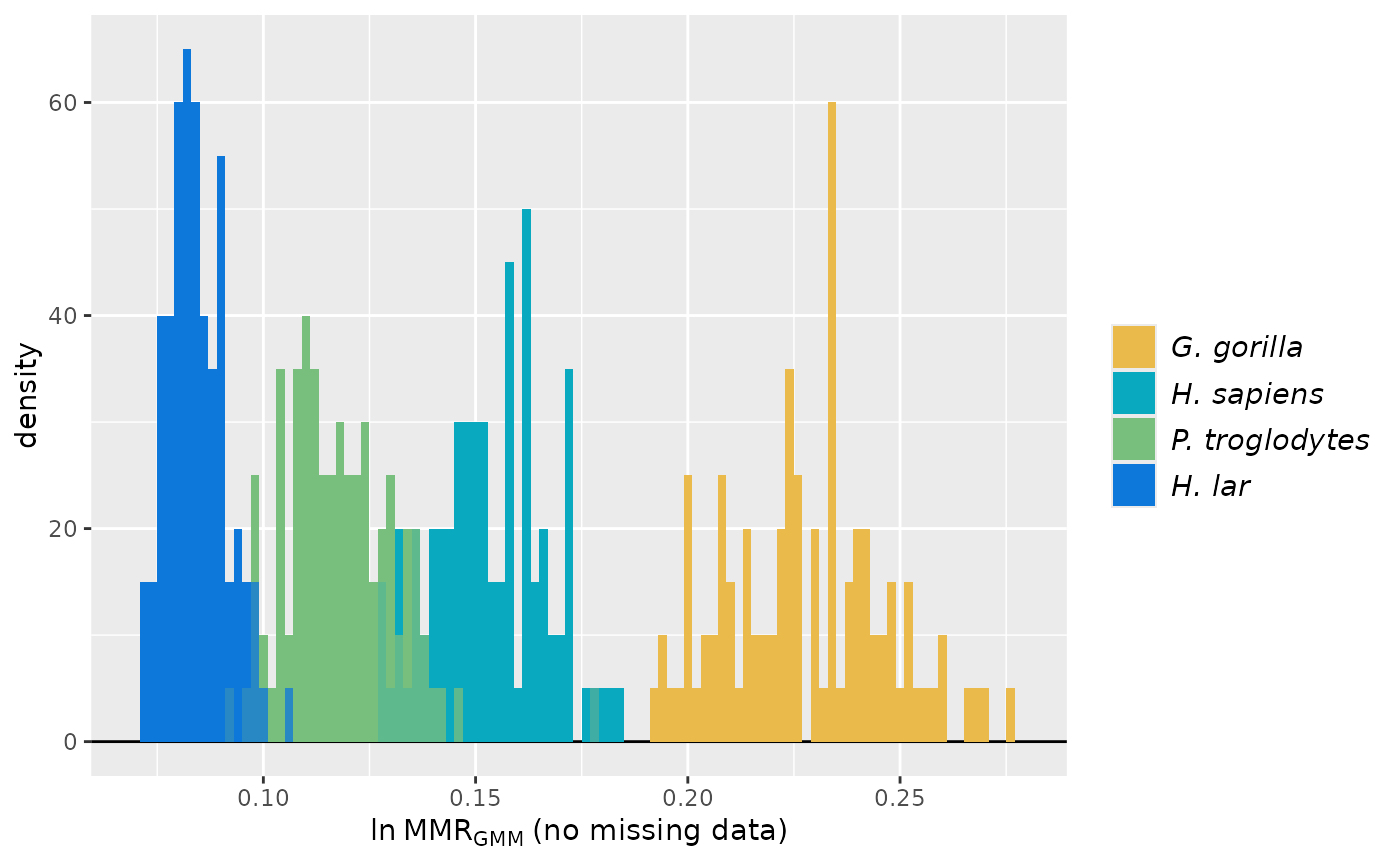 plot(test_faux_multi2, est=2, groupcols=speciescolors)
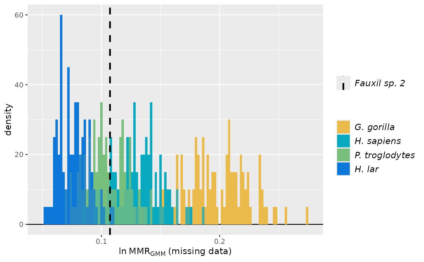 plot(test_faux_multi2, est=2, type="diff")
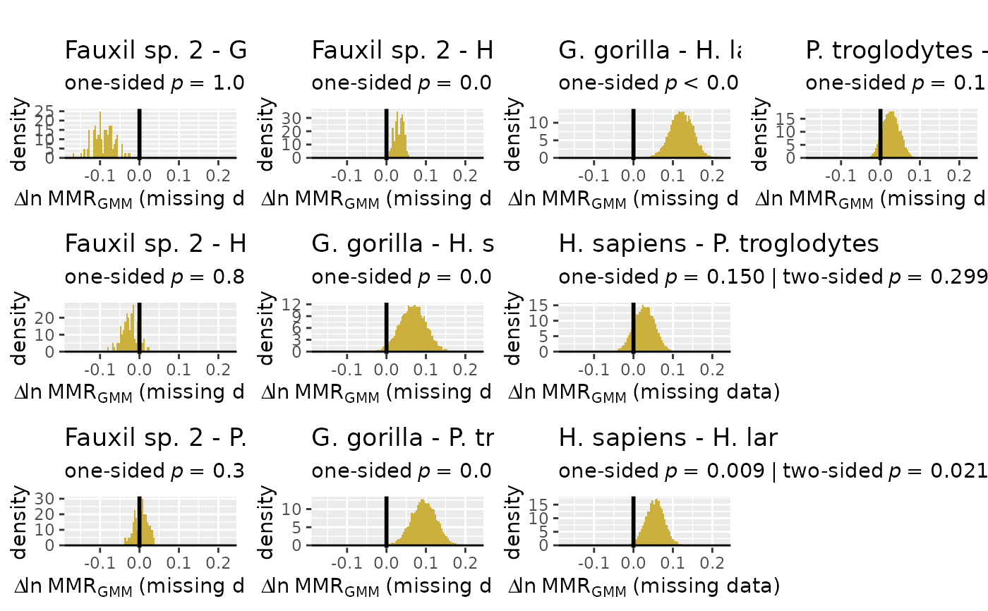 # Now the same data using a much more conservative approach by setting 'rebootstrap' to TRUE.
test_faux_multi3 <- SSDtest(
fossil=list("Fauxil sp. 2"=fauxil[fauxil$Species=="Fauxil sp. 2", SSDvars]),
comp=list("G. gorilla"=apelimbart[apelimbart$Species=="Gorilla gorilla", SSDvars],
"H. sapiens"=apelimbart[apelimbart$Species=="Homo sapiens", SSDvars],
"P. troglodytes"=apelimbart[apelimbart$Species=="Pan troglodytes", SSDvars],
"H. lar"=apelimbart[apelimbart$Species=="Hylobates lar", SSDvars]),
fossilsex=NULL,
compsex=list("G. gorilla"=apelimbart[apelimbart$Species=="Gorilla gorilla", "Sex"],
"H. sapiens"=apelimbart[apelimbart$Species=="Homo sapiens", "Sex"],
"P. troglodytes"=apelimbart[apelimbart$Species=="Pan troglodytes", "Sex"],
"H. lar"=apelimbart[apelimbart$Species=="Hylobates lar", "Sex"]),
methsUni=c("MMR", "BDI"),
methsMulti=c("GMM"),
datastruc="both",
nResamp=100,
rebootstrap=TRUE)
#> Warning: The number of possible combinations (5.47865686342759e+35) exceeds the user-specified limit. Monte Carlo sampling will be used.
#> Warning: The number of possible combinations (5.47865686342759e+35) exceeds the user-specified limit. Monte Carlo sampling will be used.
#> Warning: The number of possible combinations (5.47865686342759e+35) exceeds the user-specified limit. Monte Carlo sampling will be used.
#> Warning: The number of possible combinations (5.47865686342759e+35) exceeds the user-specified limit. Monte Carlo sampling will be used.
test_faux_multi3
#> SSDtest Object
#>
#> Comparative data set:
#> sample n female n male n unspecified
#> Fauxil sp. 2 0 0 19
#> G. gorilla 47 47 0
#> H. sapiens 47 47 0
#> P. troglodytes 47 47 0
#> H. lar 47 47 0
#> number of variables: 9
#> variable names: FHSI, TPML, TPMAP, TPLAP, HHMaj, HHMin, RHMaj, RDAP, RDML
#> SSD estimate methods (univariate):
#> MMR, BDI
#> SSD estimate methods (multivariate):
#> GMM
#> Centering algorithms:
#> geometric mean
#> Multivariate sampling with complete or missing data:
#> complete and missing
#> Number of unique combinations of univariate method, multivariate method,
#> centering algorithm, and complete or missing data structure: 4
#>
#> Resampling data structure:
#> sample n resampled data sets
#> Fauxil sp. 2 100
#> G. gorilla 100
#> H. sapiens 100
#> P. troglodytes 100
#> H. lar 100
#> resampling type
#> exact for initial resampling, then Monte Carlo for additional bootstrapping within subsamples
#> Monte Carlo for initial resampling, then Monte Carlo for additional bootstrapping within subsamples
#> Monte Carlo for initial resampling, then Monte Carlo for additional bootstrapping within subsamples
#> Monte Carlo for initial resampling, then Monte Carlo for additional bootstrapping within subsamples
#> Monte Carlo for initial resampling, then Monte Carlo for additional bootstrapping within subsamples
#> sampling
#> without replacement for initial resampling, then with replacement for additional bootstrapping within subsamples
#> without replacement for initial resampling, then with replacement for additional bootstrapping within subsamples
#> without replacement for initial resampling, then with replacement for additional bootstrapping within subsamples
#> without replacement for initial resampling, then with replacement for additional bootstrapping within subsamples
#> without replacement for initial resampling, then with replacement for additional bootstrapping within subsamples
#> missing data resampling structure:
#> sampling variable-specific number of individuals for each variable
#> number of resampled individuals by variable in each resampled data set:
#> FHSI: 8
#> TPML: 2
#> TPMAP: 5
#> TPLAP: 4
#> HHMaj: 5
#> HHMin: 2
#> RHMaj: 3
#> RDAP: 3
#> RDML: 5
#> other resampling parameters:
#> ratio variables (if present): natural log of ratio
#> matchvars = FALSE
#> na.rm = TRUE
#>
#> Median resampled estimates for each combination of methods:
#> methodUni methodMulti center datastructure Fauxil sp. 2 G. gorilla
#> 1 MMR GMM geomean complete NA 0.2246
#> 2 MMR GMM geomean missing 0.0884 0.1487
#> 3 BDI GMM geomean complete NA 0.2073
#> 4 BDI GMM geomean missing 0.0729 0.1195
#> H. sapiens P. troglodytes H. lar
#> 1 0.1525 0.1107 0.0837
#> 2 0.1097 0.0828 0.0623
#> 3 0.1472 0.1075 0.0804
#> 4 0.0895 0.0674 0.0489
#>
#> p-values (one-sided; null: first sample less or equally dimorphic as second sample):
#> MMR:GMM:geomean:complete MMR:GMM:geomean:missing
#> Fauxil sp. 2 - G. gorilla NA 0.9738
#> Fauxil sp. 2 - H. sapiens NA 0.7881
#> Fauxil sp. 2 - P. troglodytes NA 0.4363
#> Fauxil sp. 2 - H. lar NA 0.0983
#> G. gorilla - H. sapiens 0.0301 0.1544
#> G. gorilla - P. troglodytes 0.0011 0.0293
#> G. gorilla - H. lar 0.0000 0.0030
#> H. sapiens - P. troglodytes 0.0369 0.2029
#> H. sapiens - H. lar 0.0000 0.0366
#> P. troglodytes - H. lar 0.0321 0.1373
#> G. gorilla - Fauxil sp. 2 NA 0.0262
#> H. sapiens - Fauxil sp. 2 NA 0.2119
#> P. troglodytes - Fauxil sp. 2 NA 0.5637
#> H. lar - Fauxil sp. 2 NA 0.9017
#> H. sapiens - G. gorilla 0.9699 0.8456
#> P. troglodytes - G. gorilla 0.9989 0.9707
#> H. lar - G. gorilla 1.0000 0.9970
#> P. troglodytes - H. sapiens 0.9631 0.7971
#> H. lar - H. sapiens 1.0000 0.9634
#> H. lar - P. troglodytes 0.9679 0.8627
#> BDI:GMM:geomean:complete BDI:GMM:geomean:missing
#> Fauxil sp. 2 - G. gorilla NA 0.9701
#> Fauxil sp. 2 - H. sapiens NA 0.7762
#> Fauxil sp. 2 - P. troglodytes NA 0.4212
#> Fauxil sp. 2 - H. lar NA 0.0920
#> G. gorilla - H. sapiens 0.0422 0.1556
#> G. gorilla - P. troglodytes 0.0032 0.0332
#> G. gorilla - H. lar 0.0000 0.0028
#> H. sapiens - P. troglodytes 0.0416 0.2075
#> H. sapiens - H. lar 0.0000 0.0305
#> P. troglodytes - H. lar 0.0282 0.1302
#> G. gorilla - Fauxil sp. 2 NA 0.0299
#> H. sapiens - Fauxil sp. 2 NA 0.2238
#> P. troglodytes - Fauxil sp. 2 NA 0.5788
#> H. lar - Fauxil sp. 2 NA 0.9080
#> H. sapiens - G. gorilla 0.9578 0.8444
#> P. troglodytes - G. gorilla 0.9968 0.9668
#> H. lar - G. gorilla 1.0000 0.9972
#> P. troglodytes - H. sapiens 0.9584 0.7925
#> H. lar - H. sapiens 1.0000 0.9695
#> H. lar - P. troglodytes 0.9718 0.8698
#>
#> p-values (two-sided):
#> MMR:GMM:geomean:complete MMR:GMM:geomean:missing
#> Fauxil sp. 2 - G. gorilla NA 0.0762
#> Fauxil sp. 2 - H. sapiens NA 0.4081
#> Fauxil sp. 2 - P. troglodytes NA 0.9279
#> Fauxil sp. 2 - H. lar NA 0.1930
#> G. gorilla - H. sapiens 0.0383 0.3071
#> G. gorilla - P. troglodytes 0.0011 0.0780
#> G. gorilla - H. lar 0.0000 0.0183
#> H. sapiens - P. troglodytes 0.0868 0.3953
#> H. sapiens - H. lar 0.0000 0.0933
#> P. troglodytes - H. lar 0.0856 0.2861
#> BDI:GMM:geomean:complete BDI:GMM:geomean:missing
#> Fauxil sp. 2 - G. gorilla NA 0.0810
#> Fauxil sp. 2 - H. sapiens NA 0.4246
#> Fauxil sp. 2 - P. troglodytes NA 0.9025
#> Fauxil sp. 2 - H. lar NA 0.1739
#> G. gorilla - H. sapiens 0.0674 0.3164
#> G. gorilla - P. troglodytes 0.0032 0.0813
#> G. gorilla - H. lar 0.0000 0.0219
#> H. sapiens - P. troglodytes 0.0962 0.3974
#> H. sapiens - H. lar 0.0000 0.0830
#> P. troglodytes - H. lar 0.0779 0.2628
plot(test_faux_multi3, est=2, invert=1, groupcols=speciescolors)
# Now the same data using a much more conservative approach by setting 'rebootstrap' to TRUE.
test_faux_multi3 <- SSDtest(
fossil=list("Fauxil sp. 2"=fauxil[fauxil$Species=="Fauxil sp. 2", SSDvars]),
comp=list("G. gorilla"=apelimbart[apelimbart$Species=="Gorilla gorilla", SSDvars],
"H. sapiens"=apelimbart[apelimbart$Species=="Homo sapiens", SSDvars],
"P. troglodytes"=apelimbart[apelimbart$Species=="Pan troglodytes", SSDvars],
"H. lar"=apelimbart[apelimbart$Species=="Hylobates lar", SSDvars]),
fossilsex=NULL,
compsex=list("G. gorilla"=apelimbart[apelimbart$Species=="Gorilla gorilla", "Sex"],
"H. sapiens"=apelimbart[apelimbart$Species=="Homo sapiens", "Sex"],
"P. troglodytes"=apelimbart[apelimbart$Species=="Pan troglodytes", "Sex"],
"H. lar"=apelimbart[apelimbart$Species=="Hylobates lar", "Sex"]),
methsUni=c("MMR", "BDI"),
methsMulti=c("GMM"),
datastruc="both",
nResamp=100,
rebootstrap=TRUE)
#> Warning: The number of possible combinations (5.47865686342759e+35) exceeds the user-specified limit. Monte Carlo sampling will be used.
#> Warning: The number of possible combinations (5.47865686342759e+35) exceeds the user-specified limit. Monte Carlo sampling will be used.
#> Warning: The number of possible combinations (5.47865686342759e+35) exceeds the user-specified limit. Monte Carlo sampling will be used.
#> Warning: The number of possible combinations (5.47865686342759e+35) exceeds the user-specified limit. Monte Carlo sampling will be used.
test_faux_multi3
#> SSDtest Object
#>
#> Comparative data set:
#> sample n female n male n unspecified
#> Fauxil sp. 2 0 0 19
#> G. gorilla 47 47 0
#> H. sapiens 47 47 0
#> P. troglodytes 47 47 0
#> H. lar 47 47 0
#> number of variables: 9
#> variable names: FHSI, TPML, TPMAP, TPLAP, HHMaj, HHMin, RHMaj, RDAP, RDML
#> SSD estimate methods (univariate):
#> MMR, BDI
#> SSD estimate methods (multivariate):
#> GMM
#> Centering algorithms:
#> geometric mean
#> Multivariate sampling with complete or missing data:
#> complete and missing
#> Number of unique combinations of univariate method, multivariate method,
#> centering algorithm, and complete or missing data structure: 4
#>
#> Resampling data structure:
#> sample n resampled data sets
#> Fauxil sp. 2 100
#> G. gorilla 100
#> H. sapiens 100
#> P. troglodytes 100
#> H. lar 100
#> resampling type
#> exact for initial resampling, then Monte Carlo for additional bootstrapping within subsamples
#> Monte Carlo for initial resampling, then Monte Carlo for additional bootstrapping within subsamples
#> Monte Carlo for initial resampling, then Monte Carlo for additional bootstrapping within subsamples
#> Monte Carlo for initial resampling, then Monte Carlo for additional bootstrapping within subsamples
#> Monte Carlo for initial resampling, then Monte Carlo for additional bootstrapping within subsamples
#> sampling
#> without replacement for initial resampling, then with replacement for additional bootstrapping within subsamples
#> without replacement for initial resampling, then with replacement for additional bootstrapping within subsamples
#> without replacement for initial resampling, then with replacement for additional bootstrapping within subsamples
#> without replacement for initial resampling, then with replacement for additional bootstrapping within subsamples
#> without replacement for initial resampling, then with replacement for additional bootstrapping within subsamples
#> missing data resampling structure:
#> sampling variable-specific number of individuals for each variable
#> number of resampled individuals by variable in each resampled data set:
#> FHSI: 8
#> TPML: 2
#> TPMAP: 5
#> TPLAP: 4
#> HHMaj: 5
#> HHMin: 2
#> RHMaj: 3
#> RDAP: 3
#> RDML: 5
#> other resampling parameters:
#> ratio variables (if present): natural log of ratio
#> matchvars = FALSE
#> na.rm = TRUE
#>
#> Median resampled estimates for each combination of methods:
#> methodUni methodMulti center datastructure Fauxil sp. 2 G. gorilla
#> 1 MMR GMM geomean complete NA 0.2246
#> 2 MMR GMM geomean missing 0.0884 0.1487
#> 3 BDI GMM geomean complete NA 0.2073
#> 4 BDI GMM geomean missing 0.0729 0.1195
#> H. sapiens P. troglodytes H. lar
#> 1 0.1525 0.1107 0.0837
#> 2 0.1097 0.0828 0.0623
#> 3 0.1472 0.1075 0.0804
#> 4 0.0895 0.0674 0.0489
#>
#> p-values (one-sided; null: first sample less or equally dimorphic as second sample):
#> MMR:GMM:geomean:complete MMR:GMM:geomean:missing
#> Fauxil sp. 2 - G. gorilla NA 0.9738
#> Fauxil sp. 2 - H. sapiens NA 0.7881
#> Fauxil sp. 2 - P. troglodytes NA 0.4363
#> Fauxil sp. 2 - H. lar NA 0.0983
#> G. gorilla - H. sapiens 0.0301 0.1544
#> G. gorilla - P. troglodytes 0.0011 0.0293
#> G. gorilla - H. lar 0.0000 0.0030
#> H. sapiens - P. troglodytes 0.0369 0.2029
#> H. sapiens - H. lar 0.0000 0.0366
#> P. troglodytes - H. lar 0.0321 0.1373
#> G. gorilla - Fauxil sp. 2 NA 0.0262
#> H. sapiens - Fauxil sp. 2 NA 0.2119
#> P. troglodytes - Fauxil sp. 2 NA 0.5637
#> H. lar - Fauxil sp. 2 NA 0.9017
#> H. sapiens - G. gorilla 0.9699 0.8456
#> P. troglodytes - G. gorilla 0.9989 0.9707
#> H. lar - G. gorilla 1.0000 0.9970
#> P. troglodytes - H. sapiens 0.9631 0.7971
#> H. lar - H. sapiens 1.0000 0.9634
#> H. lar - P. troglodytes 0.9679 0.8627
#> BDI:GMM:geomean:complete BDI:GMM:geomean:missing
#> Fauxil sp. 2 - G. gorilla NA 0.9701
#> Fauxil sp. 2 - H. sapiens NA 0.7762
#> Fauxil sp. 2 - P. troglodytes NA 0.4212
#> Fauxil sp. 2 - H. lar NA 0.0920
#> G. gorilla - H. sapiens 0.0422 0.1556
#> G. gorilla - P. troglodytes 0.0032 0.0332
#> G. gorilla - H. lar 0.0000 0.0028
#> H. sapiens - P. troglodytes 0.0416 0.2075
#> H. sapiens - H. lar 0.0000 0.0305
#> P. troglodytes - H. lar 0.0282 0.1302
#> G. gorilla - Fauxil sp. 2 NA 0.0299
#> H. sapiens - Fauxil sp. 2 NA 0.2238
#> P. troglodytes - Fauxil sp. 2 NA 0.5788
#> H. lar - Fauxil sp. 2 NA 0.9080
#> H. sapiens - G. gorilla 0.9578 0.8444
#> P. troglodytes - G. gorilla 0.9968 0.9668
#> H. lar - G. gorilla 1.0000 0.9972
#> P. troglodytes - H. sapiens 0.9584 0.7925
#> H. lar - H. sapiens 1.0000 0.9695
#> H. lar - P. troglodytes 0.9718 0.8698
#>
#> p-values (two-sided):
#> MMR:GMM:geomean:complete MMR:GMM:geomean:missing
#> Fauxil sp. 2 - G. gorilla NA 0.0762
#> Fauxil sp. 2 - H. sapiens NA 0.4081
#> Fauxil sp. 2 - P. troglodytes NA 0.9279
#> Fauxil sp. 2 - H. lar NA 0.1930
#> G. gorilla - H. sapiens 0.0383 0.3071
#> G. gorilla - P. troglodytes 0.0011 0.0780
#> G. gorilla - H. lar 0.0000 0.0183
#> H. sapiens - P. troglodytes 0.0868 0.3953
#> H. sapiens - H. lar 0.0000 0.0933
#> P. troglodytes - H. lar 0.0856 0.2861
#> BDI:GMM:geomean:complete BDI:GMM:geomean:missing
#> Fauxil sp. 2 - G. gorilla NA 0.0810
#> Fauxil sp. 2 - H. sapiens NA 0.4246
#> Fauxil sp. 2 - P. troglodytes NA 0.9025
#> Fauxil sp. 2 - H. lar NA 0.1739
#> G. gorilla - H. sapiens 0.0674 0.3164
#> G. gorilla - P. troglodytes 0.0032 0.0813
#> G. gorilla - H. lar 0.0000 0.0219
#> H. sapiens - P. troglodytes 0.0962 0.3974
#> H. sapiens - H. lar 0.0000 0.0830
#> P. troglodytes - H. lar 0.0779 0.2628
plot(test_faux_multi3, est=2, invert=1, groupcols=speciescolors)